Click on figures for larger images.

Figure 5. U.S. Geological Survey RV Rafael with 234-kHz SWATHplus® transducers mounted on the bow. (Photograph by D. Foster, U.S. Geological Survey)

Figure 6. Maps along which Chirp sub-bottom and SWATHplus® data were collected: (A) in the northernmost St. Clair River area (sidescan-sonar data also were collected along shore-parallel tracklines); (B) at Marysville, MI; and (C) at Port Lambton, Ontario. Tracklines are shown in red. (2005 orthophoto base from Michigan State University, Remote Sensing & GIS Research and Outreach Services, USDA-FSA Aerial Photography Field Office.)

Figure 7. Map showing tracklines (red) where Boomer sub-bottom data were collected in the northernmost St. Clair River area. Tracklines are shown in red. (2005 orthophoto base from Michigan State University, Remote Sensing & GIS Research and Outreach Services, USDA-FSA Aerial Photography Field Office.)

Figure 8. The U.S. Geological Survey Mini SEABOSS, shown (left) being deployed from the RV Rafael was used to collect sediment samples, video, and digital photographs. The Mini SEABOSS components viewed from below (right) are: (A) forward video camera; (B) downward video camera; (C) video light; (D) digital still camera and housing; (E) strobe light; (F) parallel lasers for scale; (G) laser for ranging; (H) junction block; (I) Van Veen grab sampler; (J) multi-conducting cable. (Photographs by D. Blackwood, U.S. Geological Survey.)

Figure 9. Map showing location and tracklines of video drifts (red lines), locations of individual digital still photographs (green dots), and sediment-sampling locations (yellow dots) for data acquired with the Mini SEABOSS in the St. Clair River. The red dots show locations of selected observations of video along video transects from Krishnappan (2009). (2005 orthophoto base from Michigan State University, Remote Sensing & GIS Research and Outreach Services, USDA-FSA Aerial Photography Field Office.)

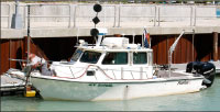
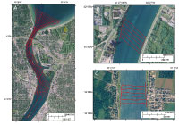
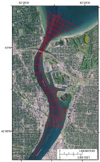
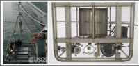
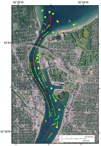
Geophysical data were collected with Chirp and Boomer sub-bottom profilers, dual-frequency sidescan sonar, and a swath-bathymetric system. Video, digital photographs, and sediment samples were collected using the USGS Mini SEABed Observation and Sampling System (U.S. Geological Survey, 2008). These systems were deployed from the RV Rafael (fig. 5), a 7.6-m USGS research vessel that is operated by the WHCMSC. Navigation data acquired during cruise operations were recoded in HYPACK®, Hydrographic Survey Software (HYPACK, Inc., 2009). Data were collected from May 29 to June 4, 2008, along tracklines spaced approximately 75 m apart in a shore-parallel orientation from 2 km south of the Black River to 1 km north of the head of the St. Clair River into Lake Huron. Tie lines were run perpendicular or at oblique angles to the shore throughout the survey area (fig. 6A). Two site-specific surveys downriver at Marysville, MI (fig. 6B), and Port Lambton, Ontario (fig. 6C), each covered approximately 500-m lengths of the river.

Swath Bathymetry and Acoustic Backscatter

Swath-bathymetric and acoustic-backscatter data were acquired with a SEA, Ltd., SWATHplus® interferometric sonar operating at a 234-kHz frequency (SEA, 2009). The SWATHplus® transducer was mounted at the bow of the RV Rafael (fig. 5). An Octopus F180 Attitude and Positioning system (Coda Octopus Group Inc., 2009) recorded ship motion (heave, pitch, roll, and yaw). Navigation was recorded with a Differential GPS (DGPS) receiver positioned directly over the SWATHplus® transducer.  Horizontal and vertical offsets between navigation and attitude antennas and the SWATHplus® transducer were recorded within the Octopus F180 and SWATHplus® configuration files; offsets were applied during acquisition.  SWATHplus® acquisition software was used to digitally log the bathymetric data at 4,096 samples per swath (ping). Bathymetric data were acquired over variable swath widths ranging from 10 to 100 m, in water depths of about 1 to 25 m.  Eight sound-velocity profiles were acquired during survey operations at roughly 4-hr intervals using an Applied Microsystems SV Plus V2 Velocimeter (Applied Microsystems, 2008). A total of 102 km of swath bathymetric data was collected.

DGPS navigation was used to record horizontal and vertical position (x,y,z) of bathymetric soundings during data acquisition aboard the RV Rafael.  Real Time Kinematic GPS (RTK-GPS) corrections were applied to the navigation data during post-processing in order to provide sub-meter horizontal and vertical accuracies of the soundings. Fort Gratiot, MI, a Continuously Operating Reference Station (CORS) (National Geodetic Survey, 2009), was used as the reference station for the RTK-GPS corrections. A “rover” RTK-GPS station was established at the tidal benchmark at the U.S. Coast Guard Base at Port Huron in order to determine the offset between North American Vertical Datum of 1988 (NAVD 88) (vertical datum referenced at the CORS site) and the International Great Lakes Datum 1985 (IGLD 85) referenced at the tidal benchmark.  The following offsets were applied to the shipboard DGPS data during post-processing: vertical offset between NAVD 88 and IGLD 85, the measured distance between the DGPS antenna and SWATHplus® transducer, and the depth of the transducer below the water line.  The resulting values were applied to the bathymetric soundings during processing to provide a measure of depth relative to IGLD 85.

SWATHPlus® and CARIS (2009) were used to process the bathymetric data.  Within SWATHplus®, data were filtered to remove spurious soundings, rectified for ship motion, and corrected for speed of sound changes within the water column, and RTK-GPS corrections were applied to the soundings to provide sub-meter vertical and horizontal accuracies for depth measurements relative to IGLD 85. The processed data were then imported to CARIS and used to generate 1-m- and 0.5-m-resolution bathymetric grids.

SwathEd (Clarke, 1998) swath-bathymetric processing software was used to extract the backscatter data from the raw SWATHplus® data files and convert these data to USGS Xsonar/Showimage file format (Danforth, 1997).  Radiometric and geometric distortions were corrected within these data following the methodology of Danforth (1997).  SwathEd was then used to generate a georeferenced acoustic backscatter mosaic at a pixel resolution of 0.5 m.  The georeferenced mosaic (UTM 17N, WGS84) was then converted to a TIFF image. A linear stretch was applied in order to enhance the dynamic range of these data.

Sidescan-sonar data were acquired with L3-Klein Associates, Inc., System 3000 dual-frequency sonar operating at 132 and 445 kHz (L3-Klein Associates Inc., 2009). Sonar data were collected at 0.033-s sampling rate, yielding a 50-m range, or 100-m swath width. L3-Klein SonarPro® acquisition software was used to log the data digitally and store them in eXtended Triton format (XTF) (Triton Imaging, Inc., 2009). The sonar system was deployed off the port side of the RV Rafael and towed less than 5 m astern.  Horizontal and vertical offsets between the sonar tow-fish and the DGPS antenna were stored within SonarPro®, allowing for tow-fish position to be calculated dynamically during acquisition. A total of 59 km of sidescan-sonar data was collected.

The sidescan-sonar data were processed following the methodology of Danforth and others (1991), Danforth (1997), and Paskevich (1992a, 1992b) to remove radiometric and geometric distortions inherent in the raw data.  Processed sonar data were then digitally mosaicked following the procedures described in Paskevich (1996) using PCI Geomatics OrthoEngine (PCI Geomatics, 2009).  The georeferenced mosaic was projected in UTM 17N coordinates, referenced to WGS84 datum at a 0.5-m pixel resolution. The mosaic was saved in TIFF format and a linear stretch was applied. The final stretched mosaic was then imported to ESRI ArcGIS (ESRI, 2009). 

Sub-bottom Profiling

Chirp sub-bottom profiles were collected using a dual-frequency (3.5 and 200 kHz) Knudsen Engineering Limited (KEL) Chirp 3200® system (Knudsen Engineering Limited, 2009). The single-beam water depths from the 200-kHz channel were logged together with navigation in ASCII format. Chirp sub-bottom data with a peak frequency of 3.5 kHz were recorded in Society of Exploration Geophysicists Y (SEG-Y) format (Barry and others, 1975) with DGPS navigation logged to the SEG-Y file trace headers. The Chirp system was fired at a rate of 0.25 or 0.5 s. The trace length was set to 67 ms. The vertical resolution of this system is approximately 30 cm. A total of 80 km of sub-bottom data was collected (fig. 6).

A Boomer system provided a higher energy source operating at 175 joules and provided deeper penetration of the sub-bottom than the Chirp system. With a peak frequency of about 1,800 Hz, the vertical resolution is approximately 1 m. The Boomer data were acquired in SEG-Y format using SonarWiz.MAP +SBP® software (Chesapeake Technology Inc., 2009). Shot-point navigation recorded DGPS location in the SEG-Y file trace headers. The layback distance from the DGPS antenna to the source and receiver was applied to the position during acquisition. The Boomer fired at a rate of 0.5 seconds and recorded each trace with 250 ms of data. A total of 58.5 km of Boomer profiles was collected (fig. 7).

Data were processed using SIOSEIS (2009) and were loaded into SeisVision™ (Halliburton, 2009) seismic-interpretation software. The major unconformities were interpreted and digitized. Isochron data were exported and subsequently imported into EarthVision® surface modeling software (Dynamic Graphics, Inc.®, 2009). The data points were gridded at a 20 x 20-m cell size. Isochron values were converted to thickness in meters using a constant sediment velocity of 1,650 m/s. This acoustic velocity correlated well depth to bedrock indicated by the geologic cross sections near the railway tunnels. We used a 5-m grid derived from our swath bathymetric data and isopach grids to calculate elevation (IGLD 85) surfaces.

Video and Photography

Video and digital photographs were collected at 37 stations using the USGS Mini SEABOSS (U.S. Geological Survey, 2008; fig. 8; fig. 9). Mini SEABOSS stations were selected based on preliminary acoustic-backscatter mosaics, with the objective of characterizing broad areas of different backscatter intensity. With the Mini SEABOSS deployed, the research vessel was allowed to drift with occasional power from the vessel to control drift direction. Continuous video was collected over a total of 11.5 km of lake and riverbed. Video drift position was derived from the HYPACK® navigation files based on the start and end times of the drift. For some portions of the drift, there was no navigation, so the position was derived from the time and position stamp in the video at 30-s intervals. The full-resolution raw video files were archived to DVD-R and were then reduced to 640 x 480 pixels and converted to MPEG-4 format.  A total of 449 photographs were obtained from a digital still camera at user-selected locations along the drifts. A Python script was used to merge drift navigation with digital photos using time of day as a common field. Positions for the digital photos were plotted (fig. 9) in ESRI ArcGIS and hot-linked to the photographs.

Sediment Sampling

Grab samples of the surficial sediment were collected at 15 stations (fig. 9), typically at the end of a drift. The upper 2 cm of sediment was scraped from the surface of the sample for texture analysis. Sediment samples were collected at locations with relatively fine-grained sediment (sand or mud). Samples were not collected in gravel or cobble areas where gravel prevented full closure of the sampler and resulted in a washed-out sample.

A total of 13 bottom samples were submitted for grain-size analysis. Two partially recovered, washed-out samples were not submitted. Grain-size analysis was performed at the USGS Sediment Laboratory at WHCMSC using methods described by Poppe and others (2005).