The following sections provide basic descriptions of methods used to collect and process the data contained in this report. Detailed descriptions of acquisition parameters, postprocessing steps, and accuracy assessments for each data type are provided within the metadata files for geospatial data layers in the appendix.

Survey Operations

Approximately 13 km² of the sea floor within Muskeget Channel and in select shore-parallel areas off Martha’s Vineyard was surveyed using the RV Rafael during USGS field activity 2010–072–FA in fall 2010 (figs. 2 and 3). An interferometric sonar was mounted on the bow of the RV Rafael to collect bathymetric data. Positioning for the ship was determined using a Communications Systems International, Inc. (CSI) LGBX Pro differential global positioning system (DGPS) antenna mounted above the cabin on the RV Rafael. Positioning for the swath bathymetry, sound velocity profiler at the sonar head, and attitude were determined by using a CodaOctopus F180 DGPS antenna mounted on a rigid, vertical pole approximately 3 m above the swath transducers. A NovAtel DL–V3 real-time kinematic (RTK) antenna, also mounted above the swath transducers, was used to acquire water-level heights for tidal corrections. Vessel positions were recorded to HYPACK, Inc. hydrographic survey software.

During acquisition, the RV Rafael maintained speeds between 1.5 and 2.5 m/s. Data were collected along tracklines spaced approximately 70 m apart. Trackline spacing was designed to ensure overlap of adjacent interferometric swaths.

Interferometric-Sonar Bathymetry

Nearly 227 km of interferometric data were collected with a Systems Engineering and Assessment, Ltd. (SEA) SWATHplus-M 234-kilohertz interferometric-sonar system during USGS field activity 2010–072–FA (fig. 3). This field activity was divided into two surveys. Data collected from October 12 to 19 fall within the scope of Survey 1. Data collected on November 16 fall within the scope of Survey 2. Select tracklines from Survey 1 were reoccupied during Survey 2 to provide data on bedform migration and sea-floor morphologic change. Equipment configurations and acquisition parameters were the same for both surveys.

Vessel motion (heave, pitch, roll, and yaw) was recorded simultaneously with the swath data using a CodaOctopus F180 attitude and positioning system. The SWATHplus transducers and F180 unit were mounted on the RV Rafael on a rigid vertical pole, with the F180 mounted on top of the SWATHplus transducers, at a depth of approximately 0.5 meter (m) below the sea surface. The speed of sound at the transducer face was monitored continuously with an AML Oceanographic Micro SV velocimeter mounted at the sonar heads. Horizontal and vertical offsets between the antennae and the F180 and SWATHplus transducers were applied and recorded in the F180 and SWATHplus configuration files. DGPS navigation was used to record horizontal and vertical positions of the soundings during acquisition. Real-time kinematic corrections were transmitted to a DGPS receiver on the survey vessel once every second from a base station. RTK vertical heights were used to correct tidal offsets during postprocessing.

Acquisition of bathymetric data was performed with SWATHplus acquisition and processing software (Swath Processor). Vessel motion data recorded by the F180 were used to correct for heave, pitch, roll, and yaw of the vessel, and filters were applied to remove spurious soundings. Sound velocity profiles (SVP) of the water column were acquired with an AML Oceanographic SV Plus V2 hand-deployed velocimeter. Profiles were collected at least once during each survey day and multiple times per day when the data suggested significant stratification within the water column. Sound velocity profiles were applied within the SWATHplus software during processing to correct bathymetric soundings for errors resulting from changes in the speed of sound within the water column. Cast locations, graph images, and text data files for each profile are available for download in the appendix.

Following acquisition, soundings were imported into CARIS hydrographic information processing system (HIPS) software for further processing. RTK-corrected water-level-height values were merged with the line files to reference soundings to mean lower low water (MLLW), and remaining spurious soundings were removed by further filtering and by manual swath editing. Continuous bathymetric surfaces for Survey 1 and Survey 2 were created at 2-meter-per-pixel (mpp) grids and exported from CARIS in ASCII format for import into Esri grid format (fig. 4). Figure 5 shows a three-dimensional view of Muskeget Channel from data collected during Survey 1, as seen in QPS Fledermaus software (version 7), with a fivefold- vertical exaggeration to highlight sea-floor topography. Figure 6 shows a grid of the difference between Survey 1 and Survey 2 for a section of sea floor covered in bedforms. In general, the bedforms in this area migrated between 10 and 15 m to the south during a 1 month period.

Acoustic Backscatter

Swath interferometric backscatter was extracted from the raw bathymetric data and processed to produce a backscatter mosaic image from the data collected during the first survey (fig. 7). Following acquisition in Swath Processor, interferometric backscatter data were imported into Chesapeake Technology's SonarWiz (version 5). Altitudes were selected using an automated bottom tracker with minor adjustments using manual digitizing. An empirical gain normalization function was applied to the backscatter within SonarWiz to optimize the dynamic range and enhance the quality of the mosaic. A 24-bit gray-scale GeoTIFF image of backscatter was produced at 1.0-mpp resolution. Backscatter data were acquired along approximately 169 km of trackline during Survey 1, yielding a total mosaic area of about 13 km² (fig. 7). Backscatter data for Survey 2 are not included in the appendix, but can be made available upon request.

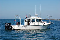
Figure 2. Photograph showing the configuration of acquisition equipment on the U.S. Geological Survey research vessel Rafael. The real-time kinematic global positioning system antennae and the swath interferometric-sonar head are located off the bow. Photograph by Dave Foster.

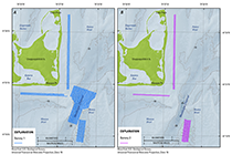
Figure 3. Map showing tracklines along which bathymetric depth data were collected surrounding Muskeget Channel, Massachusetts. Two separate surveys were conducted so that morphologic changes could be assessed within an area of large bedforms and along potential cable routes. Data from A, Survey 1 were collected in October 2010 and B, Survey 2 were collected in November 2010. Is., Island; Pt., Point.

Figure 4. Map showing shaded-relief bathymetry collected within the vicinity of Muskeget Channel, Massachusetts. Two separate surveys were conducted so that morphologic changes could be assessed within an area of large bedforms and along potential cable routes. Data from A, Survey 1 were collected in October 2010 and B, Survey 2 were collected in November 2010. Coloring represents depth in meters relative to mean lower low water. Is., Island; Pt., Point.

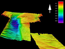
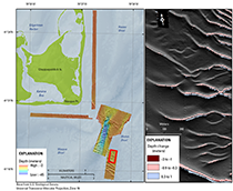
Figure 5. Map showing shaded-relief bathymetry of Muskeget Channel, Massachusetts, in three dimensions. These data were collected during a survey conducted in October 2010. Vertical exaggeration is sixfold.

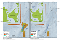
Figure 6. Map showing shaded-relief bathymetry collected within the vicinity of Muskeget Channel, Massachusetts, during a survey conducted in October 2010. Inset map is showing the change in bathymetry for a select area between Survey 1 in October 2010 and Survey 2 in November 2010. Pink and red tones indicate erosion and blue tones indicate deposition. Gray areas (hillshaded) are within ±30 centimeters and below instrument accuracy. Bedform migration is between 10 and 15 meters within the inset area, and net sediment transport is to the south. Is., Island; Pt., Point.

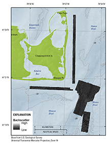
Figure 7. Map showing acoustic-backscatter intensity collected within the vicinity of Muskeget Channel, Massachusetts, during a survey conducted in October 2010. Backscatter intensity is an acoustic measure of the hardness and roughness of the sea floor. In general, high values (light tones) represent rock, boulders, cobbles, gravel, and coarse sand. Low values (dark tones) generally represent fine sand and muddy sediment. Is., Island; Pt., Point.