

Groundwater Quality and Geochemistry of the Western Wet Gas Part of the Marcellus Shale Oil and Gas Play in West Virginia
Links
- Document: Report (8.52 MB pdf) , HTML , XML
- Appendixes:
- Appendix 1 (78.1 KB xlsx) - Correlation matrix showing Spearman’s correlation coefficients of statistical significance at a confidence interval of 99 percent for 58 variables, including 45 chemical constituents, 4 principal component analysis scores, 8 land use classifications, and well depth
- Appendix 1 (18.4 KB zip) - In CSV format
- Data Release: USGS data release - Dataset of C1-C6 dissolved trace hydrocarbon measurements in the western “Wet Gas” part of the Marcellus Shale Oil and Gas Play in West Virginia, U.S.A. collected between June and August 2018
- NGMDB Index Page: National Geologic Map Database Index Page (html)
- Download citation as: RIS | Dublin Core
Acknowledgments
The U.S. Geological Survey (USGS) would like to acknowledge Brian A. Carr of the West Virginia Department of Environmental Protection, and William Toomey and Scott Rodeheaver of the West Virginia Department of Health and Human Resources for their assistance in providing support to bring this study to fruition. Todd Cooper, Keith Robinson, and Rick Shaver of the West Virginia Department of Health and Human Resources are also acknowledged for assisting with field reconnaissance of sampling sites, assisting with sampling of the sites discussed in this report, and providing daily assistance with transporting samples for shipment to the USGS National Water Quality Laboratory in Denver, Colorado. Finally, the USGS would like to acknowledge the residents of northwestern West Virginia who allowed access to their wells for sampling. This study would not be possible without the endeavors of the aforementioned individuals.
Abstract
Thirty rural residential water wells in the wet gas region of the Marcellus Shale oil and gas play in northwestern West Virginia were sampled by the U.S. Geological Survey (USGS) in 2018, in cooperation with West Virginia State agencies, to analyze for a range of water-quality constituents, including major ions, trace metals, radionuclides, bacteria, and methane and other dissolved hydrocarbon gases. The groundwater-quality data collected for this study were used to assess the overall quality of groundwater in the study area in relation to public drinking-water standards. The groundwater-quality data were also evaluated with respect to geology, well depth, topographic setting, and proximity to oil and gas wells to identify possible relations to these factors.
The presence of total coliform bacteria in groundwater is a potential indicator of surface contamination. The presence of Escherichia coli bacteria is indicative of fecal contamination of groundwater from either human or animal sources and may be considered an indicator of other related pathogens such as viruses. Total coliforms were detected in 26 of the 30 (87 percent) wells sampled. Eleven of the 30 (37 percent) wells sampled had detections of Escherichia coli bacteria.
Sodium concentrations in 24 of 30 (80 percent) samples exceeded the U.S. Environmental Protection Agency (EPA) 20-milligram per Liter (mg/L) health-based value (HBV). Manganese, aluminum, and iron concentrations exceeded the EPA 50, 2.0, and 300 micrograms per liter (μg/L) secondary maximum contaminant level (SMCL) drinking-water standards at 14 (47 percent), 7 (23 percent), and 5 (17 percent) of the 30 wells sampled. Two of the 30 (7 percent) wells sampled had concentrations of manganese that exceeded the 300-µg/L USGS health-based screening level (HBSL). Arsenic concentrations at 7 of 30 (23 percent) wells sampled exceeded the 10-μg/L EPA maximum contaminant level (MCL) health-based drinking water standard. The EPA maximum contaminant level goal (MCLG) for arsenic is 0 μg/L and 29 of 30 wells sampled contained detectable concentrations of arsenic.
None of the 30 wells sampled exceeded the U.S. Office of Surface Mining Reclamation and Enforcement (OSMRE) 28-mg/L immediate action level (IAL) for methane in groundwater and only 1 of 30 (3 percent) sites exceeded the 10-mg/L OSMRE level of concern (LOC) for methane in groundwater. Of the 28 wells sampled for radon-222 all 28 (100 percent) exceeded the EPA proposed 300-picocuries per liter (pCi/L) MCL for radon. None of the samples exceeded the 4,000-pCi/L alternate maximum contaminant level (AMCL) which is applicable to public drinking water systems that have adopted radon mitigation programs.
Wilcoxon Signed Rank Tests indicated statistically significant differences at a 95 percent confidence interval (p less than 0.05) in radium-226, barium, and ethane groundwater concentrations with respect to the density of oil and gas wells present within a 500-meter (m) radius around the rural residential wells sampled for the study. Samples from residential wells that had four or fewer oil and gas wells in the surrounding 500-m radius had statistically lower concentrations of radium-226, bromide, and ethane than samples from residential wells sampled that had five or more oil and gas wells in the surrounding 500-m radius. Given the available data, the relationship between concentrations of radium-226, bromide, and ethane for wells sampled in this study and oil and gas development or natural geochemical processes is not clear.
Groundwater-age tracers (chlorofluorocarbons, tritium, and sulfur hexafluoride) were sampled at 17 of the 30 wells. All 17 samples contained a fraction of young, post-1950s groundwater. Many of the groundwater samples collected for this study have high calcium to sodium ratios and low total dissolved solids concentrations, indicating they are dominated by recently recharged water. A subset of samples had chloride to bromide mass ratios between 70 and 200, indicating that deep Appalachian basin brines mixed with the shallow groundwater. For most of the samples in this study, the C1 through C6 hydrocarbons have characteristics that reflect a biogenic gas signature that has, to varying degrees, undergone oxidation processes during transport. None of the samples show a characteristic thermogenic cracking pattern among the hydrocarbon ratios.
Introduction
West Virginia’s northwestern oil and gas field is an area of about 2,733 square miles (mi2) in parts of 14 counties in northwestern West Virginia (fig. 1) and has been the focus of unconventional oil and gas production from the Marcellus Shale since 2004. A previous study of the groundwater and surface-water quality of the Marcellus Shale oil and gas play in West Virginia focused on a part of the play that was dominated by methane, commonly referred to as “dry gas,” production in the Monongahela River basin (Chambers and others, 2015). The current study focused on an eight-county area (fig. 1) of intense oil and gas drilling and production in a part of the Marcellus Shale play in West Virginia that contains a higher proportion of longer chain hydrocarbons such as ethane, pentane, butane, propane, and hexane, commonly referred to as “wet gas.” Oil and gas have been produced from the region since 1859, when oil production began in the Burning Springs field of Wirt County (Hennen, 1911). The area is one of the most intensely developed areas of hydrocarbon production from the Marcellus Shale oil and gas play in West Virginia. Production in this field began just after production in the Drake field in Pennsylvania. The Drake field included the oldest well purposely drilled to produce oil in the United States (Hennen, 1911).
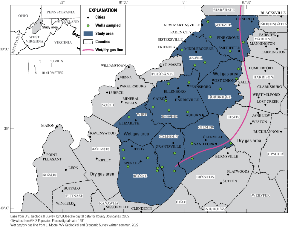
Location of study area and distribution of sites sampled within the wet gas dominated part of the Marcellus Shale oil and gas play in northwestern West Virginia.
Recent studies by the Centers for Disease Control and Prevention (CDC) and other entities have shown that the mortality and morbidity rates for a variety of serious, chronic conditions, such as diabetes, heart disease, and some forms of cancer in Appalachia, a region of the Appalachian Mountains which extends from New York to Alabama and includes parts of 12 States, are higher than elsewhere within the United States (Hendryx and Ahern, 2009). Causes of the increased mortality and morbidity are not clear, but factors such as poor diet, high rates of smoking, and other socioeconomic factors may contribute to the higher-than-average morbidity and mortality rates in the region. To date, groundwater quality in areas of active oil and gas production from the Marcellus Shale has not been fully assessed to determine the effect, or lack thereof, of oil and gas drilling, production, and transport on the quality of groundwater used for drinking water supply in the region.
A study to address the quality of groundwater in northwestern West Virginia was conducted during 2018–20 by the U.S. Geological Survey (USGS) in cooperation with the West Virginia Department of Health and Human Resources and the West Virginia Department of Environmental Protection, with grant support from the CDC. A major goal of this study was to assess current groundwater quality in areas of active and legacy oil and gas production as part of a baseline assessment of groundwater quality. Another goal was to assess groundwater quality as a potential factor with respect to the increased mortality and morbidity in northwestern West Virginia. Groundwater data collected for this study may be used by the CDC and linked with epidemiologic and health data to further investigate potential factors responsible for higher-than-average morbidity and mortality in the region.
Purpose and Scope
Groundwater-quality data, reports, and information are sparse for the counties in northwestern West Virginia that are experiencing intense development of oil, gas, and other hydrocarbons, and were not adequate to assess and characterize the quality of groundwater within the study area.
To address this data gap, 30 rural residential water wells were sampled in 2018 for a broad range of chemical constituents. This study focused on rural residential water supplies in areas with a high density of oil and gas drilling, production, and pipeline transport to provide a baseline dataset of groundwater quality for current assessment and future comparison.
The groundwater samples were analyzed for chemical and physical properties, including nutrients, major ions, trace elements and metals, indicator bacteria, radionuclides, and methane and other dissolved hydrocarbon gases. The groundwater-quality data and summary statistics are presented to assess current groundwater-quality conditions in the region and are compared to drinking-water standards. In addition, the data were analyzed using multivariate statistical methods to assess potential correlations with geology, topographic setting, well depth, and proximity to oil and gas wells. Mineral saturation indices (SIs) were calculated to better understand reduction-oxidation (redox) and other geochemical processes that control groundwater quality. Principal component analysis was used to identify processes affecting groundwater quality and associations among dissolved constituents in groundwater. Concentrations of methane and other dissolved hydrocarbon gases were analyzed to help determine potential sources of, and potential processes affecting, methane and other dissolved hydrocarbon gases in groundwater. Groundwater ages determined from various tracers are presented and a conceptual model for the evolution of groundwater quality is discussed.
Description of Study Area
The study area for this investigation is within the Marcellus Shale oil and gas play in northwestern West Virginia and includes parts of 8 counties (Wetzel, Tyler, Doddridge, Ritchie, Wirt, Calhoun, Gilmer, and Roane) covering approximately 2,498 mi2 (fig. 1) and is completely within the Appalachian Plateaus Physiographic Province (Fenneman, 1938; Fenneman and Johnson, 1946). In 2017, the 8-county area produced 913,899 thousand cubic feet (MCF) of natural gas, 3,023,712 barrels (bbl) of oil, and 4,495,150 bbl of natural gas liquids (wet gas; table 1; West Virginia Geological and Economic Survey, 2020a). Oil and gas production is greater in the northern part (Wetzel, Tyler, Doddridge, and Ritchie Counties) than in the southern part (Wirt, Calhoun, Gilmer, and Roane Counties) of the eight-county study area.
Table 1.
Oil, gas, and natural gas liquids production in 2017 in the 8-county study area comprising the wet-gas-dominated part of the Marcellus Shale play in northwestern West Virginia.[Data are available from the West Virginia Geological and Economic Survey (2020a). MCF, thousand cubic foot; >, greater than; —, data unnecessary for analysis; bbl, barrel]
The study area consists of rugged, moderately incised hilly terrain with uplifted plateaus capped by resistant layers of relatively flat-lying sandstone and shale. Approximately 57,452 oil and gas wells are present in the 8-county study area as of 2021, some of which are active and others which are no longer producing or have been abandoned (West Virginia Geological and Economic Survey, 2020b).
Average annual precipitation for the study area, based on 1991–2020 station normals (table 2) for the National Weather Service weather station in Middlebourne, West Virginia (town of Middlebourne is shown on fig. 1), is 47.27 inches per year (in/yr). Maximum and minimum monthly temperatures for the station are 84.1 degrees Fahrenheit (°F) in July and 19.4 °F in January (National Oceanic and Atmospheric Administration, 2022). Precipitation is typically distributed unevenly with respect to topography, with areas at higher elevations typically receiving higher average amounts of precipitation than areas at lower elevations.
Table 2.
Long-term precipitation and temperature data for 1991–2020 station normals at the National Weather Service weather station in Middlebourne, West Virginia.[Data accessed July 27, 2021 at https://www.ncdc.noaa.gov/cdo-web/datatools/normals. Jan., January; Feb., February; Mar., March; Apr., April; Jun., June; Jul, July; Aug., August; Sep.; September; Oct., October; Nov., November; Dec., December; °F; degrees Fahrenheit; in., inch]
Public supplies are the principal source of water for 61.7 percent of residents and businesses in the study area. These public water supplies serve 41,478 people and account for 4.86 million gallons per day (Mgal/d) of freshwater withdrawals (2.0 Mgal/d of groundwater and 2.86 Mgal/d of surface water) for residential and commercial use. The remaining water use consists of 3.02 Mgal/d of groundwater withdrawals for residential and commercial supply and serves an estimated 37,774 people who rely on private domestic wells or other unregulated sources such as springs (table 3; U.S. Geological Survey, 2020). Rural residential water systems, primarily from individual wells, supply 38.3 percent of all water used for residential and commercial use in the study area. The majority of water used for public supply in the region (58.8 percent) is derived from surface-water sources, primarily from stream withdrawals, and the remaining part (41.2 percent) is derived from groundwater withdrawals. For rural residential homeowners, however, almost 100 percent of their withdrawals are derived from groundwater (private wells or springs).
Table 3.
2015 water-use data for the 8-county area comprising the study area, the wet gas dominated part of the Marcellus Shale oil and gas play in northwestern West Virginia.[Water-use data are for 2015 and were retrieved from the U.S. Geological Survey National Water Information System website (NWIS-Web) database (U.S. Geological Survey, 2020). Mgal/d, million gallons per day]
Hydrogeologic Setting and Groundwater Flow
The generalized hydrogeologic framework of the study area is based on regional topography, stratigraphy, and structure, with upland plateaus formed by resistant clastic rocks and valleys developed in zones of structural weakness. Pennsylvanian clastic rocks form the predominant units cropping out in the uplands and valley walls of southern and central West Virginia (Cardwell and others, 1968). Geologic nomenclature used in this report is that of the West Virginia Geological and Economic Survey (2022). The study area is underlain by Pennsylvanian and Permian stratigraphic units that consist of gently dipping, relatively flat lying, slightly folded, interbedded sandstone, conglomerate, siltstone, shale, and coal, with local beds of limestone and dolomite. Mapped geologic units within the study area (fig. 2) consist of three geologic groups or formations and include the Monongahela Formation and Conemaugh Group of Pennsylvanian age and the Dunkard Group of Permian and Pennsylvanian age (Cardwell and others, 1968). The bedrock units commonly are overlain by a relatively thin layer of regolith or alluvium (Berg and others, 1980). Older sedimentary rock formations of Pennsylvanian age, including the Allegheny and Kanawha Formations, have been mapped to the southeast of the study area (fig. 2).
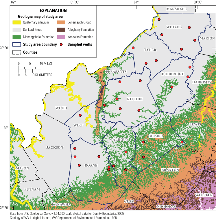
Geology of the study area and location of rural residential wells sampled within the wet gas dominated part of the Marcellus Shale oil and gas play in northwestern West Virginia.
Although the lithology of the various geologic units which form the fractured-bedrock aquifers within the study area are similar in composition to each other, there is some variability between them (Blake and others, 2002). The oldest rocks, which crop out in the southeastern part of the study area, are those of the Glenshaw and Casselman Formations of middle to upper Pennsylvanian age and comprise the Conemaugh Group (fig. 2). The Monongahela Formation crops out within the central part of the study area and is of upper Pennsylvanian age. The youngest rocks are those of the Waynesburg and Washington Formations of upper Pennsylvanian to Permian age and comprise the Dunkard Group, cropping out in the northwestern part of the study area (fig. 2). The proportion of shale, limestone, sandstone, coal, and other sedimentary rocks varies from one formation to another; it is this variability in lithologic composition that can result in varying groundwater quality within the study area.
In West Virginia, the Conemaugh Group consists of the Casselman Formation and underlying Glenshaw Formation, the border between units being the top of the Ames Limestone Member (Milici, 2004; U.S. Geological Survey and Association of American State Geologists, 2020b). The Monongahela Formation consists of the Gilboy Sandstone Member, Little Captina Limestone Member, McKeefrey Siltstone Member, Morningview Sandstone Member, Redstone Member, and Ritchie Red Beds (U.S. Geological Survey and Association of American State Geologists, 2020b). The Dunkard Group consists of interbedded sandstones, limestones, shales, and coal beds of the Washington and Greene Formations (Fedorko and Skema, 2013).
The proportion of limestone to other lithologies within the Monongahela Formation and Dunkard Group is greater than in the Conemaugh Group. There also are differences in the depositional sequence for the various formations. The older Pennsylvanian-age rocks in southern West Virginia were deposited in an area that received more paleorainfall and paleorecharge; thus, the sulfur content was diluted compared to the younger Pennsylvanian- and Permian-age rocks in northern West Virginia, which formed in a drier paleoclimate with higher ash, nutrient, and dissolved solids content that collectively resulted in higher sulfur content (Cecil and others, 1985). The younger rocks were deposited in marine environments that had greater contents of sulfur and calcium carbonate. There is also a difference in the depositional sequence for the limestone, with the limestones within the Monongahela Formation and Dunkard Group primarily deposited in non-marine brackish environments and the older rocks of the Conemaugh Group deposited in marine environments (Cardwell and others, 1968).
Groundwater-flow paths in the study area are relatively short and limited to two principal aquifers: (1) unconsolidated, unconfined, alluvial aquifers composed of sand, silt, clay, and gravel in valley settings, and (2) fractured-bedrock aquifers composed of siliciclastic and carbonate sedimentary rocks and associated coal (Puente, 1985). Because they tend to be shallow and thin, the alluvial aquifers within the study area typically are not used for water supplies but can combine with soil and regolith to provide shallow storage for recent recharge. Fractured-bedrock aquifers are the primary aquifers in the study area. Regolith is commonly thin with low permeability, providing little groundwater storage. Groundwater storage and flow in bedrock occurs through joints, fractures, and bedding-plane separations (Kozar and Mathes, 2001). In the study area, secondary permeability due to jointing and stress-relief fracturing accounts for most of the porosity and permeability in the bedrock because the original intergranular porosity commonly has been filled by calcium carbonate or silica cementation (Wyrick and Borchers, 1981).
Recharge to fractured-bedrock aquifers in the region occurs primarily as rainfall (Puente, 1985). Snowmelt is only an important source of recharge in areas of West Virginia at elevations above 3,000 feet (ft), but the maximum elevation in the study area is only 1,680 ft. Once precipitation falls on the surface, the part that does not run off to streams percolates into and through shallow soils and regolith and eventually recharges fractured-bedrock or alluvial aquifers. A decrease in hydraulic conductivity with depth in bedrock aquifers in the region has been documented by several researchers. For a mine site in West Virginia, the average hydraulic conductivity of an aquifer decreased from 3.3 × 10⁻⁴ ft per second (ft/s) at a depth of 150 ft to 3.3 × 10⁻⁸ ft/s at depths greater than 328 ft (Bruhn, 1985). For a site in Greene County, Pennsylvania about 60 miles from the study area, hydraulic conductivity decreased by an order of magnitude per 100 ft of depth to a depth of approximately 500 ft (Stoner, 1983). According to Callaghan and others (1998), the vast majority of groundwater circulation in Appalachian Plateau settings occurs at moderate depths of less than 300 ft.
In the Appalachian Plateaus, local fractured-bedrock aquifers of less than 5.0 mi2 are defined by topographic valleys and boundary ridges, with total relief of only a few hundred feet from valley bottoms to ridge tops, on average. Each small valley may contain a locally distinct aquifer (Kozar and others, 2020) from which groundwater discharges to a nearby stream or to deeper subregional or regional aquifers (fig. 3). The ridges surrounding the valley define the lateral boundaries of the local aquifer and its principal recharge area. Subregional aquifers (generally from 100 to 500 ft below land surface [bls]) occur at intermediate depths between the shallow local aquifer (less than 500 ft bls) and deeper regional aquifers. Subregional aquifers are larger than local aquifers and may include several smaller local aquifers. Discharge of groundwater from subregional aquifers is primarily to tributary streams with drainage areas typically much larger than 5.0 mi2. A small component of recharge to these subregional aquifers is from deeper regional aquifers that typically discharge to large rivers. Depth to saline water (brines) has been used to infer the base of regional aquifers (Callaghan and others, 1998). In West Virginia, the depth to brackish water ranges from more than 2,000 ft near the southern part of the study area to a minimum of less than 50 ft in areas bordering the Ohio River (Foster, 1980).
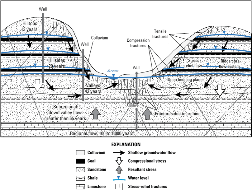
Conceptual model of shallow groundwater flow in an unmined Appalachian Plateaus fractured bedrock aquifer, including apparent age of groundwater.
Within the local aquifers, groundwater typically flows from hilltops to valleys, approximately perpendicular to local tributary streams, through an intricate network of stress-relief fractures and interconnected bedding-plane separations, commonly in a stair-step pattern (fig. 3; Wyrick and Borchers, 1981; Harlow and LeCain, 1993). Vertical hydraulic conductivity can be negligible within the clastic sedimentary rocks comprising the aquifer, resulting in approximately horizontal groundwater flow parallel to bedding (especially within coal beds) that discharges as springs or seeps in hillsides and valleys (Harlow and LeCain, 1993). A small proportion of the groundwater flows deeper within the central core of the mountain or ridge, especially within coal beds and along bedding-plane separations, and likely reaches the valley to discharge locally to surface water or may recharge subregional and regional aquifers (Kozar and others, 2012). Groundwater flow in valleys primarily occurs in bedding-plane separations beneath valley floors and in vertical and horizontal stress-relief fractures along valley walls (Wyrick and Borchers, 1981). Enhanced permeability of bedrock in valleys may result in groundwater flow parallel to and beneath local tributary streams before ultimately discharging to surface-water bodies.
This study is focused on shallow groundwater quality in the wet gas dominated part of the Marcellus Shale oil and gas play in northwestern West Virginia (fig. 4), where the Marcellus Shale does not crop out but is present at depths greater than 7,000 ft bls. The Marcellus Shale ranges in depth from approximately 7,500 ft bls in Wetzel County, West Virginia, where rocks dip slightly, to 8,200 ft bls in the central trough of the Robinson Run Syncline in Doddridge County, based on published geologic cross sections (Ryder and others, 2009). The Marcellus Shale ranges from less than 20 ft thick in the western part of the study area to a maximum of 60 ft in the eastern portion of the study area (fig. 5). Multi-lateral horizontal production wells can produce very large quantities of gas from even thin shale reservoirs.
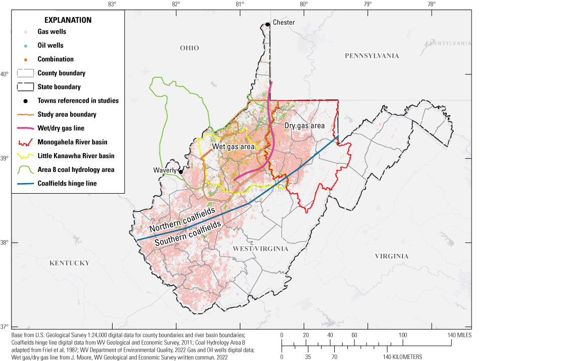
Map showing the distribution of oil and gas wells in West Virginia and the line separating the wet gas and dry gas dominated parts of the Marcellus Shale oil and gas play in the study area for this investigation.
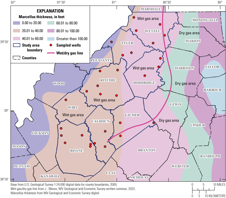
Map showing the thickness of the Marcellus Shale within the wet gas dominated part of the Marcellus Shale oil and gas play in northwestern West Virginia.
The yield of water from residential wells completed within the study area has long been postulated to be a function of topography, specifically the dominance of stress-relief fractures in the valleys and hillsides and the absence of such fractures on the hilltop settings (Wyrick and Borchers, 1981). Stress relief fracturing processes were documented for a study conducted at Twin Falls State Park in Wyoming County, West Virginia (Wyrick and Borchers, 1981) and are often referenced in hydrogeologic literature for the Appalachian region. For this study, well depth and well yield data for 482 water wells in the eight counties in northern West Virginia coincident with the geographic area for this study fully support the stress relief fracturing concepts of Wyrick and Borchers (1981), which were based on earlier work by Ferguson (1967). Data for the 482 wells were retrieved from the U.S. Geological Survey National Water Information System (NWIS) Groundwater Site Inventory (GWSI) database (table 4; U.S Geological Survey, written commun., 2019). Contact the USGS National Water Information System (NWIS) local data manager for the Virginia and West Virginia Science Center to request the quality control data referenced in this report. Those data and topographic assessment from digital elevation models (DEMs) show distinct differences with respect to topographic setting—wells in valleys have higher mean yields (35.6 gallons per minute [gal/min]) than wells on hillsides (29.0 gal/min) or hilltops (7.6 gal/min). Well depths were deeper on hilltops with an average depth of 173 ft compared to hillsides (average depth of 119 ft) or valley wells (average depth of 72 ft). Hilltop, hillside, and valley wells had median specific capacities of 0.72, 0.64, and 5 gallons per minute per foot (gal/min/ft) of drawdown, respectively. It should be noted that the data retrieved from the NWIS database (U.S Geological Survey, 2020) for the evaluation by Wyrick and Borchers (1981) are older and likely reflect past drilling practices that may not represent modern drilling methods. One example of this includes the fact that wells drilled with older cable tools typically are much shallower than wells drilled with modern air rotary methods. The data do, however, support the stress relief fracture theory, although overall trends are not as distinct with respect to the three topographic settings as was evident for similar data from southern West Virginia where topography is much steeper and overall relief from valley bottoms to hilltops is greater.
Table 4.
Well depth, well yield, and specific capacity data for 482 wells in the 8-county study area comprising the wet gas dominated part of the Marcellus Shale oil and gas play in northwestern West Virginia.[Data retrieved from the USGS Groundwater Site Information database (GWSI) database (U.S Geological Survey, written commun., 2019). ft, foot; bls, below land surface; gal/min, gallon per minute; gal/min/ft, gallon per minute per foot of drawdown]
Median groundwater ages determined by chlorofluorocarbon (CFC) analysis for hilltop, hillside, and valley bedrock wells in a similar hydrogeologic setting in the Monongahela River basin (which is immediately to the east of the study area), were typically on the order of 44, 31, and 35 years, respectively, whereas groundwater ages for wells sampled in West Virginia’s low-sulfur coal region in southern West Virginia were on the order of 18, 28, and 26 years, respectively (McAuley and Kozar, 2006). Relatively older groundwater is likely for wells sampled in the study area, which is adjacent to the Monongahela River basin, as compared to wells sampled in southern West Virginia, which has higher relief, steeper gradients, and much more distinct differences in topography. Longer residence time gives groundwater more time to interact with minerals in the bedrock, potentially affecting groundwater quality. The lack of clear topographic control on groundwater age in the study area may be related to the topography which is characterized as a rolling hummocky-type terrain, and therefore the distinction between hilltops, hillsides, and valleys is less prominent in northern West Virginia where total relief between ridge tops and streams is typically only 200–300 ft compared to southern West Virginia where total relief can be as much as 1,000 ft.
The Burning Springs Anticline in Wirt and Ritchie Counties is indicative of a location where hydrocarbons naturally discharge to the surface and is an area where hydrocarbons were historically skimmed from the surface of Oil Creek before modern well technology to drill deeper oil and gas wells was developed (Hennen, 1911; Eggleston, 2004). A series of freshwater and saline water maps for West Virginia (Foster, 1980) indicate that depth to saline water within the study area is typically very shallow, ranging from a minimum of 50-ft bls close to the western margin of the study area in Wetzel County bordering the Ohio River to a maximum of 750 ft in the eastern part of the study area in Calhoun County. Such shallow depths are within the depth range for rural residential water wells.
Land Cover and Land Use
Land cover in the study area is predominately forested or scrub shrub areas and represents 2,379 mi2 (87 percent) of the study area. Residential and urban areas occupy approximately 15 mi2 (0.5 percent). Barren land and developed open space account for 131 mi2 (5 percent), 197 mi2 (7 percent) is pasture, grassland, or cultivated crops, and open water and wetlands occupy 11 mi2 (0.5 percent; Homer and others, 2015). The rural region has one dominant industry—oil and gas production. The study area has been developed extensively for oil and gas since 1859 (Eggleston, 2004). Approximately 57,452 oil and or gas wells have been drilled within the study area, including 1,626 multi-lateral horizontal Marcellus Shale oil and gas wells (fig. 6).
Recent data for the study area indicate that what little coal mining is occurring is primarily in Wetzel County, with a few permitted mines in Roane, Doddridge, and Gilmer Counties (West Virginia Geological and Economic Survey, 2020c). Many of these mines are inactive as indicated by 2019 coal production data, which indicates that coal mining is only active in Wetzel County within the study area (West Virginia Office of Miner’s Health Safety and Training, 2020). In 2019, underground coal mines in Wetzel County produced 6,497,707 tons of coal.
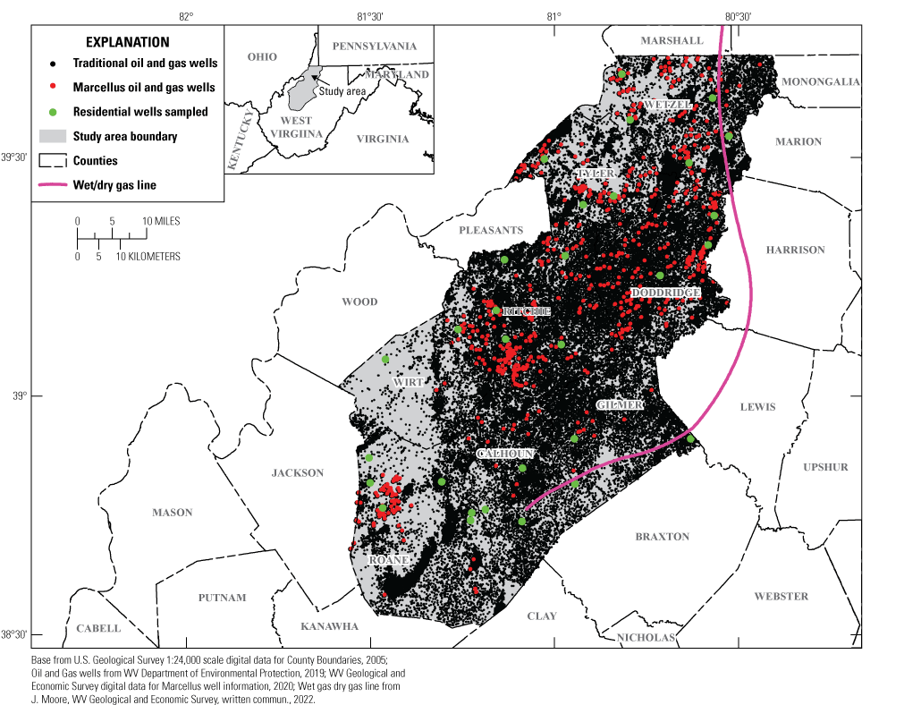
Map showing the distribution of oil and gas wells and rural residential water wells sampled for this study within the wet gas dominated part of the Marcellus Shale oil and gas play in northwestern West Virginia.
Previous Investigations
Recent investigations of groundwater quality within the study area are limited but include Chambers and others (2012, 2015) and Harkness and others (2017). Harkness and others (2017) conducted a comprehensive study of the geochemistry of naturally occurring methane and saline groundwater in an area of unconventional shale gas development and the results are similar to those of this study. In fact, the study areas for the two studies overlapped significantly and both studies collected data in Doddridge, Ritchie, Tyler, and Wetzel Counties, West Virginia. Harkness and others (2017) collected 145 groundwater samples from 105 wells in the aforementioned counties and in Harrison County, West Virginia. In addition to sampling a large number of wells over a 5-county area in northwestern West Virginia where legacy and more recent Marcellus Shale oil and gas production has occurred, that study also analyzed for a broad array of isotopic data that were not collected for our investigation. The Harkness and others (2017) study monitored geochemical variations of drinking-water wells before, during, and after the installation of nearby shale gas wells and concluded that there was no indication of groundwater contamination and subsurface impact from shale-gas drilling and hydraulic fracturing within the study area. The study also found that saline groundwater was common and indicative of an upward flow of Devonian-age brines migrating into shallow aquifers and were modified by water-rock interactions. Occurrence of ethane, propane, and carbon isotope ratios of ethane indicate that thermogenic gas contributes to the overall mixture of natural gas in shallow aquifers in the study area. Dissolved gas in shallow groundwater, however, predominantly contained microbial methane, even though both biogenic and migrated thermogenic gases occur in shallow groundwater in the study area but are unrelated to shale gas development. That study did document surface water contamination that occurred in Tyler County from two injection well sites and a flowback spill related to shale gas development.
A USGS statewide assessment of groundwater quality within West Virginia (Chambers and others, 2012) indicated that Pennsylvanian and Permian fractured-bedrock aquifers, which are typical of the current study area, can have elevated concentrations of radon-222, a carcinogenic and radioactive gas known to cause lung cancer. The highest concentrations of radon-222 documented in the statewide assessment were for wells sampled in the Blue Ridge Physiographic Province in Jefferson County in the easternmost part of West Virginia. However, median radon-222 concentrations also were commonly elevated in wells sampled in Permian and Pennsylvanian age bedrock aquifers and typically exceeded the EPA proposed 300-picocurie per liter (pCi/L) maximum contaminant level (MCL) drinking water standard. Other than radon, the statewide study did not find chemical constituents of concern for wells sampled within the general area of study for this investigation.
A water-quality assessment of stream base flow and groundwater in the Marcellus Shale oil and gas play within the Monongahela River basin, an area immediately to the east of the current study area, was conducted in 2011 and 2012 (Chambers and others, 2015). The 2011–12 study was conducted prior to high intensity development of the Marcellus Shale oil and gas play to provide a baseline of groundwater and stream base flow data for future comparison. The principal groundwater findings of the previous study were based on 39 wells and 2 springs sampled June through September of 2011.
Principal components analysis conducted for the 2011–12 study specify that the first principal component indicates gradients of redox conditions and dissolved solids concentrations with strong negative loadings for sodium, bromide, chloride, fluoride, barium, total dissolved solids, specific conductance, pH, and methane, which are inversely proportional to dissolved oxygen, carbon dioxide, argon, nitrogen, and redox potential. These gradients may reflect a continuum from deeper waters with higher concentrations of sodium, bromide, chloride, fluoride, barium and methane (constituents typically found in higher concentrations in deeper brines) to shallow, more dilute, more recent waters with higher concentrations of dissolved atmospheric gases. Whether this continuum reflects a typical gradient from recharge from shallow groundwater to deeper groundwater or indicates other pathways resulting in mixing of shallow groundwater and deeper brines is unknown.
The second principal component had strong positive loadings for calcium, magnesium, potassium, iron, manganese, sulfate, total dissolved solids, specific conductance, argon, nitrogen, carbon dioxide, and hardness, and negative loadings for geologic age, methane, redox potential, bromide, and dissolved oxygen (Chambers and others, 2015). The second component reflects a gradient from conditions typical of shallow groundwater in the Appalachian region, which have high concentrations of total dissolved solids, iron, manganese, calcium, magnesium, and sulfate, to conditions more typical of deeper groundwater. Carbonate dissolution and reduction of pyrite and siderite are dominant processes in the shallow aquifers of the region and can result in elevated concentrations of total dissolved solids, iron, manganese, calcium, and sulfate, whereas higher concentrations of chloride and bromide are more common in deeper waters.
Dissolved gas analyses for the 2011–12 study indicate that the majority of sites (38 of 41) sampled were from a shallow groundwater source. Analysis of groundwater data collected for the study with respect to geologic structure, including wells located near deep through-going faults, did not reveal a clear pattern linking methane concentrations to the presence of geologic structure.
Other prior work focused on hydrogeology, brines and salt in waters, areas affected by coal mining, or basin studies. An assessment of groundwater hydrology of the Little Kanawha River in West Virginia (Hobba, 1980) provided a preliminary assessment of groundwater quality and water-well yields in the basin. Well yields were classified by topographic setting and median well yields ranged from a minimum of less than 1 gallon per minute (gal/min) on hilltops to 14 gal/min in valleys adjacent to the stream side of wide terraces. The report included a map of specific capacity in gallons per minute per foot (gal/min/ft) of drawdown showing areas with groundwater development potential in three categories: less than 2, 2–5, and greater than 5 gal/min/ft. The map also summarized groundwater quality for 795 previously collected water-quality samples and 48 samples collected for the project. Water samples from the 48 sites were analyzed for pH, silica, calcium, magnesium, sodium, potassium, bicarbonate, carbonate, chloride, fluoride, sulfate, nitrate, aluminum, iron, manganese, hardness, and total dissolved solids (TDS), and included maps showing the suitability of groundwater for residential and public supply in the basin.
One of the more comprehensive assessments for a part of the study area was an assessment of groundwater hydrology of the alluvial and bedrock aquifers bordering the Ohio River between Chester and Waverly, West Virginia (Bader and others, 1997), an area immediately to the west of the current study area. Well yields in fractured-bedrock aquifers ranged from 1 to 300 gal/min, with a median of 6 gal/min. Groundwater samples were compared to U.S. Environmental Protection Agency (2019) drinking-water standards. Eight percent of the wells sampled contained chloride concentrations in excess of the 250-milligrams per liter (mg/L) U.S. Environmental Protection Agency (EPA) SMCL drinking water standard for aesthetic effects such as taste, odor, and color. Iron and manganese concentrations ranged from 3 to 52,000 μg/L and from less than 1 to 1,900 μg/L, respectively. Median iron concentrations were 50 micrograms per liter (μg/L) in alluvial aquifers and 16 μg/L in fractured-bedrock aquifers. Median manganese concentrations were 510 μg/L in alluvial aquifers and 56 μg/L in fractured-bedrock aquifers. Arsenic, barium, mercury or phenol were detected at concentrations exceeding EPA drinking-water standards at 7 of the 50 wells sampled. The hardness of the water exceeded 120 mg/L in 91 percent of the samples, which is characteristic of hard to very hard groundwater which can cause scaling of water lines, boilers, hot water heaters, and water distribution systems.
An inventory and assessment of salt water produced in conjunction with oil and gas development in the Little Kanawha River basin of West Virginia, which is immediately southeast of the study area, was conducted (Kirwan and Rauch, 1988) prior to the advent of horizontal well drilling methods. Based on data from 1981 to 1984, their study estimated that 4.2 × 10⁷ gallons (gal) of salt water had been produced as part of oil and gas development in the watershed, and of that amount, 2.6 × 10⁷ gal had been disposed of as surface discharge, either on land or in streams. The 2.6 × 10⁷ gal of saltwater approximated 11.9 percent of the chloride and 1.7 percent of the TDS load within the Kanawha River during the period assessed.
A report on Appalachian connate water (Heck and others, 1964) provides a discussion of connate brines in West Virginia, Pennsylvania, and Ohio. Two additional reports provide a discussion of oil and gas resources in Pleasants, Wood, and Ritchie Counties (Haught, 1955) and Doddridge and Harrison Counties (Haught, 1959) in West Virginia. None of the reports provided information on the quality or quantity of potable groundwater for residential or public groundwater supplies.
The first salt well completed in West Virginia was completed in Kanawha County in 1812. In 1815 at Charleston, West Virginia gas was first encountered while drilling for salt (Eggleston, 2004). In 1859, the Rathbone brothers bored a salt well on burning Springs Run, but rather than encountering salt, they hit petroleum at a depth of 200 feet—which produced 200 barrels a day (Eggleston, 2004). The first purposely drilled well for oil in West Virginia was completed along the Burning Springs Anticline in Wirt County in 1860 by the Rathbone brothers and is known as the Rathbone well (Hennen, 1911). The well was begun in the later part of 1859 and was completed in May of 1860 to a depth of 303 ft and produced oil at a rate of 100 barrels per day (Hennen, 1911). Prior to that, oil was skimmed off the surface of Oil Springs Creek. Discovery of oil and gas produced one of the earliest oil and gas booms in the United States. The natural occurrence of salt water and hydrocarbons at shallow depths in the basin is common, especially along the Burning Springs Anticline, and both oil and gas production and natural flow of brines and hydrocarbons have the potential to locally affect groundwater and surface-water quality within the basin. The report contains several illustrations depicting the conceptual understanding of groundwater flow and interaction of fresh and saline water within the basin.
A study of the hydrology of the U.S. Office of Surface Mining Reclamation and Enforcement (OSMRE) Area 8 Eastern Coal Province in West Virginia and Ohio (Friel and others, 1987), which includes the entire current study area, assessed the quality of groundwater and surface water in an area of limited coal mining activities. About 1 million tons of coal were mined from 26 surface mines and about 6.7 million tons from 6 underground mines in the Area 8 Coal Province in 1980. Coal mining has declined within the study area in recent years (West Virginia Office of Miner’s Health Safety and Training, 2020; West Virginia Geological and Economic Survey, 2020c) and oil and gas production, including prolific development of the Marcellus Shale oil and gas play has increased (West Virginia Geological and Economic Survey, 2020b). Based on samples collected from 158 streams within the Area 8 Eastern Coal Province study area, the median specific conductance of surface water was 260 microsiemens per centimeter (μS/cm) and ranged from 41 to 4,035 μS/cm; the median pH was 7.3 standard units and ranged from 2.9 to 8.1; alkalinity ranged from 4.8 to 2,845 mg/L, with a median of 35.5 mg/L; total iron concentrations ranged from 100 to 565,000 μg/L, with a median of 630 μg/L; and dissolved manganese concentrations ranged from 10 to 5,100 μg/L, with a median of 64 μg/L. Dissolved iron and sulfate concentrations were highest in streams draining mined areas. Water well yields assessed in the study ranged from less than 1 to 350 gal/min. Highest median iron concentrations were from streams draining coal mined areas and were 16 times higher than for streams draining unmined areas.
An assessment of water resources of the Little Kanawha River basin in West Virginia provided a comprehensive evaluation of both groundwater and surface water resources within the basin, both with respect to water quality and water quantity (Bain and Friel, 1972). Average annual streamflow of the river was 3,100 cubic feet per second (ft3/s) or 1.35 cubic feet per second per square mile (ft3/s/mi2) and recharge to groundwater was calculated to be between 5 and 7 in/yr. Water in the Little Kanawha River and its tributaries are a calcium carbonate type of water. Wells inventoried for that project ranged in yield from 1 to 8 gal/min, with median yields in the Dunkard Group, Monongahela Formation, and Conemaugh Group fractured-rock aquifers of 7.0, 6.5, and 4.0 gal/min, respectively. Potable groundwater exists to depths less than 200 ft in the western part of the basin and to depths between 500 and 1,000 ft in the eastern part of the basin. The 1972 report contains maps of chemical constituent distribution including pH, iron, chloride, and hardness.
Methods of Data Collection and Analysis
The factors considered in designing the sampling protocol, selecting sampling sites, and the methods used for statistical analysis of the water-quality data collected for this study are discussed in the following sections of the report. Methods utilized for sample collection and analysis of a broad range of water-quality constituents, including field measured parameters of pH, specific conductance, dissolved oxygen, and water temperature, indicator bacteria (Escherichia coli [or E. coli] and total coliform), common ions (including calcium, sodium, magnesium, and potassium), trace metals (including iron, manganese, and arsenic), nutrients (nitrate, nitrite and orthophosphate), dissolved gases (including nitrogen, argon, and helium), dissolved hydrocarbons (including methane and ethane), age dating constituents (including chlorofluorocarbons, sulfur hexafluoride, and tritium) are discussed. Design of the quality assurance and quality control (QA/QC) protocols used are also discussed, as are the methods used for statistical and graphical analysis, and geochemical modeling of the data collected for the project.
Selection of Sampling Sites
Sampling site selection was based primarily on two criteria. First, sites were selected to provide data from areas of active or legacy oil and gas production in northwestern West Virginia in areas of current Marcellus Shale gas, oil, and natural gas liquids (NGL) production. Second, sites were selected in areas with sparse groundwater-quality data in northwestern West Virginia. Surficial geology, which commonly is used as a site selection criterion, was not an important factor for site selection in this study. Most of the study area has surficial geology within the Pennsylvanian to Permian age Dunkard Group (50 percent), the Pennsylvanian age Conemaugh Group (22 percent), or the Monongahela Formation (16 percent), all of which have similar lithologies. To a lesser extent, the study area’s surficial geology is within the Allegheny Formation (10 percent) and there are minor exposures of the Kanawha Formation and Quaternary alluvial deposits (1 percent each).
Sample Collection
Groundwater samples were collected from 30 residential water wells in the study area from June 11 to July 18, 2018, by the USGS using standard USGS methods (Wilde and others, 2004; U.S. Geological Survey, 2006). Prior to sampling, wells were purged to remove standing water from the well and ensure that representative water samples were collected. Wells were purged for a sufficient period to allow pH, dissolved oxygen, specific conductance, and water temperature to stabilize, and then water samples were collected and processed. Prolonged 3-volume purging of the wells was not required because the wells sampled were primarily rural residential wells with submersible pumps and are purged daily as part of routine use. Methods applicable for low-yield wells were utilized at a few wells to avoid pulling the water level down to the pump intake, which can cause turbidity issues, aerate the sample water, and potentially damage the well pump. Periodic water-level measurements were made and served as the criteria for length of the well purge in conjunction with close monitoring of dissolved oxygen, pH, water temperature, and specific conductance using a multiparameter water-quality sonde, which was calibrated daily.
For the wells sampled, plumbing and well-casing materials included steel, galvanized steel, polyvinyl chloride (PVC), and other plastics. The purging procedure minimized potential contamination from the well casing and plumbing, as non-contaminating Teflon sample tubing was connected as close to the wellhead as possible, usually at the pressure tank, prior to any treatment such as a water softener or chlorinator, and pumps were kept running as much as possible to prevent sample contamination from the plumbing or backflow from holding tanks. The sample line was then fed to a manifold with sampling ports and a port for connection of a multiparameter water-quality sonde. Field properties were measured in the flowthrough apparatus and monitored until parameters stabilized prior to sampling. To prevent environmental contamination, samples typically were collected and processed inside a mobile field laboratory or a portable processing chamber assembled near the closest spigot on the plumbing system to the well prior to any water treatment equipment such as chlorinators or water softeners, typically at the pressure tank.
Samples for bacterial analysis were collected and processed according to standard USGS methods (Myers and Sylvester, 2014) and processed using the Colilert system (IDEXX, 2019) according to established methods (American Public Health Association, American Water Works Association, and Water Environment Foundation, 2018), a defined substrate liquid-broth medium method for determination of total coliform bacteria and E. coli. Water samples for bacterial analysis were collected by cleansing the spigot on the pressure tank or water valve on the discharge line from the pump with isopropyl alcohol; the spigot then was allowed to thoroughly dry before filling a pre-sterilized 100-milliliter (mL) sample bottle. Bacteria samples were processed within 2 hours of collection and incubated for 24–28 hours, according to USGS standard protocols.
All samples from the 30 wells were analyzed for field properties (pH, water temperature, specific conductance, and dissolved oxygen), turbidity, alkalinity, major ions, metals, trace elements, total coliform and E. coli. bacteria, uranium, radium-226, radium-228, and gross alpha and gross beta radiation (table 5). Radon-222 was analyzed for samples from 28 of the 30 wells (two samples were lost in shipment). A subset of samples from 17 of the 30 wells were collected for analysis of dissolved hydrocarbons, sulfur hexafluoride (SF6), CFCs, deuterium, oxygen-18, tritium, and helium as a methods development process for a secondary but related pilot study for a new USGS dissolved hydrocarbons and isotope laboratory established concurrent with this study in Reston, Virginia. Samples were processed according to standard USGS protocols (Wilde and others, 2004). Measurements of water temperature, specific conductance, dissolved oxygen concentration, pH, turbidity, and alkalinity were made on site at the time of sampling.
Table 5.
Constituents and reporting limits for major ions, metals, trace elements, nutrients, radionuclides, fecal indicator bacteria, and dissolved hydrocarbons analyzed in groundwater samples collected from sites in the wet gas dominated part of the Marcellus Shale oil and gas play in northwestern West Virginia.[μg/L, microgram per Liter; mg/L, milligram per Liter; col/100 mL, colony per 100 milliliters; ng/kg, nanograms per kilogram; pCi/L, picocurie per Liter pg/kg; picogram per kilogram; fg/kg, femtogram per kilogram; E. coli, Escherichia coli; µS/cm, microsiemens per centimeter; —, no data entered]
Quality Assurance and Quality Control
Three types of QA/QC samples were collected during the project—field blanks, equipment blanks, and replicates. Replicates were run on environmental samples to assess the reproducibility of analytical methods and assess bias that may have resulted in the laboratory analysis. Field blanks were run to assess any contamination that may have resulted from field sampling methods, to evaluate decontamination procedures between sites, and to detect contamination on sampling equipment during transit to or from the sampling site. Equipment blanks were collected in the laboratory at the USGS office in Charleston, West Virginia, and field blanks were run in the field to assess the potential of contamination from blank water used to process field and equipment blanks, the deionized water and detergent solutions used to decontaminate equipment between sampling sites, and to assess whether residual contamination was being carried over from site to site. All quality assurance data for the water samples collected for this study are stored in the quality assurance part of the USGS quality of water data (QWDATA) database for West Virginia (U.S. Geological Survey, written commun., 2022).
Variability for a replicate sample pair was quantified by calculating the relative percent difference (RPD) of the samples. The RPD was calculated using the following formula
where R1 is the concentration of the analyte in the first replicate sample and R2 is the concentration of the analyte in the second replicate sample. Concentrations of replicate sample pairs differed by small amounts, typically less than 15 percent of the RPD. Constituents with higher RPD were typically constituents at low concentrations at or below the method detection limit. Analytical or sampling variability was considered minimal as a result.CFC, SF6, Tritium, Dissolved Gas, and Dissolved Hydrocarbon Sampling
Samples for CFCs, SF6, tritium, and dissolved gas analysis were collected according to procedures described by the USGS Groundwater Dating Laboratory (https://water.usgs.gov/lab). The CFC samples were collected in 125-mL glass bottles with metal foil sealed caps. The SF6 samples were collected in 1-L borosilicate amber glass bottles with polycone seal caps. Tritium samples were collected in 500-mL high density polyethene bottles with polycone seal caps. Dissolved gas samples were collected in pairs in pre-weighed 125-mL bottle pairs with butyl rubber septa. After sampling, the dissolved gas bottles were stored on ice and refrigerated until analysis to minimize bacterial activity. The CFC, SF6, and dissolved gas bottles were purged and filled under water to prevent contamination from outside air.
Dissolved hydrocarbon samples were collected by filling a 1-L bottle to overflowing in a bucket then allowing a minimum of three volumes of sample water to flush through the sample bottle. The bottle was then removed from the water and three potassium hydroxide preservative tablets were added to the sample and the sample bottle was capped and taped shut. Samples were kept chilled in a cooler and then transferred to a refrigerator, prior to shipment to the USGS Groundwater Dating Laboratory in Reston, Va.
Analysis of Water Chemistry
Major ions, nutrients, metals, trace elements, and radon-222 were analyzed using standard EPA or USGS methods at the USGS National Water Quality Laboratory in Denver, Co. Trace elements and common ions, such as calcium, magnesium, sodium, potassium, iron, manganese, sulfate, chloride, bromide, and fluoride, were analyzed by inductively coupled plasma (ICP) mass spectrometry; nutrients (nitrate + nitrite, nitrite, total nitrogen, and orthophosphate) were analyzed by digestion or colorimetric methods; and radon-222 was analyzed by liquid scintillation methods. Reporting limits for these analyses are provided in table 5.
CFC, SF6, and Dissolved Gas Analysis
CFCs (CFC-11, CFC-12, and CFC-113), SF6, and dissolved gas samples for nitrogen, argon, methane, carbon dioxide, and oxygen analysis were shipped to the USGS Groundwater Dating Laboratory in Reston, Va. for analysis using gas chromatography methods (Busenberg and Plummer, 1992, 2000).
Tritium Analysis
Tritium samples were processed in the USGS Groundwater Dating Laboratory using Helium-3 (3He) ingrowth analysis using methods similar to those described by Schlosser and others (1988) and Papp and others (2012). For ingrowth, 500-gram (g) water samples were transferred in 1-L volume stainless steel vessels fitted with vacuum-tight copper tube stubs. The samples were on a vacuum manifold with a pressure of less than 1×10⁻⁴ torr, created by a stainless-steel liquid nitrogen trap and a rotary vane pump removing air-sourced 3He below the limits of detection. After degassing, the samples were clamped and then stored for at least 6 months to allow for tritium to decay to 3He. After the ingrowth interval, the canisters were attached to an automated vacuum manifold for 3He extraction and analysis on Thermo Scientific Helix SFT Split Flight Tube mass spectrometer. On the manifold, the 3He and any residual gases were extracted from the canisters, the gases were removed with cryogenic traps and reactive getters, and the 3He was quantitatively captured on a Gifford-McMahon cycle cryocooler with charcoal matrix at less than 10 Kelvin (K). The 3He from tritium decay was then expanded into the Helix SFT for analysis. The 3He samples were calibrated against samples of air of known 3He abundance and samples were corrected for any residual air-sourced 3He in the ingrowth canisters. Analysis of replicate samples and blind intercomparison showed method precision better that 1 percent relative standard deviation (RSD) and a lower reporting limit of 0.01 tritium unit (TU).
Dissolved Hydrocarbon Analysis
Dissolved hydrocarbon concentrations were analyzed by the USGS Dissolved Gas Laboratory. The dissolved C1 to C6 hydrocarbons (methane, ethane, ethene, ethyne, propane, propene, propyne, n-butane, isobutane, 1-butene, n-pentane, isopentane, 2- and 3-methylpentane, hexane, and benzene) were analyzed using a custom purge and trap gas chromatography-flame ionization detector and atomic emission detector (GC-FID/AED) system developed for quantifying trace volatile gases in water. This analytical method is sensitive to trace constituents in the picomole range, while maintaining enough dynamic range to enable quantification of samples with considerable amounts of dissolved gas and has been employed in numerous studies where trace hydrocarbon concentrations are of interest (Haase and others, 2014; Cozzarelli and others, 2017; Orem and others, 2017; Kozar and others, 2020). Duplicate samples for dissolved hydrocarbons were collected in 1-L borosilicate glass bottles, as discussed above, and refrigerated until analysis to inhibit bacterial activity and degassing. Dissolved hydrocarbon data for this study are published in a USGS data release (Haase and others, 2022).
The dissolved hydrocarbon analytical system was calibrated using a suite of certified gas standards with blend accuracies greater than 10 percent. Additionally, quality control samples consisting of homogenized tap water, nitrogen-purged water, and water purged with air containing parts-per-million to parts-per-billion by volume mixing ratios of hydrocarbon gases were collected in the laboratory in a manner identical to the field samples and analyzed to verify analytical performance (Haase and others, 2022). Methane was quantified exclusively on the flame ionization detector (FID) because concentrations are typically much higher than other hydrocarbons (Prinzhofer and others, 2000). The FID detection limit is 4.97 nanograms per kilogram (ng/kg) and the calibration precision is 0.9 percent RSD. The C2 to C6 hydrocarbons were simultaneously measured on the atomic emission detector (AED) and the FID, with the reported value coming from the highest sensitivity detector that was still in the range of linearity, which was typically the AED for most measurements of these compounds. The detection limits of the AED are typically in the range of 6.75 to 25.1 × 10⁻³ ng/kg, with calibration precisions between 1 and 14 percent, replicate quality control samples had concentration RSDs between 4 and 10 percent, and median percent differences between duplicate field samples were 2 to 56 percent.
Geospatial Analysis
Geospatial analysis for this project was conducted by incorporating requisite project data into ArcGIS version 10.6 (Esri, 2020). Data layers compiled or created for the ArcGIS Arc-Map project included but were not limited to (1) the locations of water wells sampled during the project, (2) locations of current and legacy vertical and more recent horizontal oil and gas wells, (3) a geologic map of the study area, and (4) significant geographic features such as locations of public water lines, roads, streams, cities, towns, county boundaries, and land use. The primary tasks of the spatial analysis were to determine (1) the extent of oil and gas well production near the sampled residential water wells (within either a 500-m or 1,000-m radius) in the study area, and (2) the geologic formation in which the sampled water wells were completed. Thus, GIS was used to determine the extent of oil and gas production and geology surrounding each residential water well sampled, which were the primary factors considered to potentially affect groundwater quality in the study area, although other factors, such as well depth and topographic setting, also were evaluated as part of the study.
Statistical and Graphical Analysis
Statistical and graphical techniques were used to summarize and compare water chemistry and field parameters among different sites according to spatial location, geology, proximity to oil and gas wells, and topographic setting. Statistical analyses were conducted and graphics were created with the R statistical computing environment version 3.4.0 (R Core Team, 2017). Non-parametric techniques were used for computing descriptive and multivariate statistics from water-quality data that were, in some instances, censored at multiple levels. Censored data are low-level concentrations of chemicals with values between zero and the laboratory’s reporting limit. The robust regression on order statistics (ROS) survival analysis method was used to calculate summary statistics for censored data because of the relatively small sample sizes and to avoid transformation bias of non-normal water-quality data (Helsel, 2012). Scatter plots were used to understand the relation between ion concentrations, mineral saturation indices, and pH. Tukey-type boxplots, censored at the highest reporting limit (Lorenz, 2018) were created to understand the relation between water quality and site characteristics, whereas trilinear Piper diagrams (Piper, 1944; Back, 1966) were used to show a graphical representation of major ion chemistry. Boxplots and Piper diagrams were created with the USGS smwrGraphs R package and, when necessary, the robust ROS method was employed to impute values for censored water-quality data (Lorenz and Diekoff, 2017). For statistical analysis, data for the wells sampled in the Conemaugh Group and Monongahela Formation were combined for multivariate statistical analysis because of the low sample size (only 7 and 4 wells sampled in the Monongahela Formation and Conemaugh Group, respectively), but were graphed as separate units in the boxplots and trilinear diagrams. Hillside and hilltop wells were also combined and labeled as upland wells for multivariate statistical and graphical analysis.
Prior to multivariate statistical analysis, and because of the presence of multiple censoring levels, censored data were re-coded to u-Scores with the codeU function in the USGS smwrQW package (Lorenz, 2018). The u-Score is the sum of the sign of the differences between each value and all other values and is equivalent to the rank but scaled so the median is equal to zero. Using u-Scores allows for the computation of multivariate relations without requiring censoring at the highest reporting limit and retains information at multiple reporting limits. In cases where a column of data has only one censoring level, the u-Scores are the same as ordinal methods of ranking for one reporting limit (Helsel, 2012).
Principal components analysis (PCA) was used to identify relations between the major chemical and hydrological processes that could explain dissolved element concentrations in the water-quality dataset. Principal component analysis is a multivariate statistical analysis method that allows rapid analysis of large datasets and extracts the eigenvectors and eigenvalues from a covariance matrix. It can be used to understand the intercorrelations of many variables and provide insight into underlying hydrogeochemical processes (Davis, 1986). PCA was computed with the principal function in the R psych package (Revelle, 2022), which first computes correlation coefficients (Spearman’s rho) for the raw u-Scores and then performs a PCA on the resulting correlation matrix (app. 1). Varimax rotation was applied to simplify the structure of the PCA model, which maximized the differences in components and aided in the interpretation of results. Water-quality variables that had missing values or were censored in more than 40 percent of the values were excluded from the PCA. The variable loadings from the varimax-rotated PCA were used to determine the master variables for each rotated component. Resulting loadings from the PCA and statistically significant correlations (p less than 0.01) from the correlation matrix were retained and used for further interpretation of the dataset.
The Wilcoxon Signed Rank Test (Helsel, 2012) was run to determine whether there were statistically significant differences between (1) the geologic formations, (2) the topographic setting (uplands or valleys) in which the water wells are present, (3) the depth of water wells sampled (less than 95 ft in depth or greater than or equal to 95 ft in depth), and (4) with respect to the number of oil and gas wells in proximity to the water wells sampled for the study (pre-1930 oil and gas wells, Marcellus Shale oil and gas play wells only, and oil and gas wells within 500 or 1,000 m of residential water wells sampled for the study). For the Wilcoxon Signed Rank Test, p less than 0.05 was used to determine if differences between groups of data are statistically significant. When p is less than 0.05, it indicates that groups are statistically different from one another, whereas if p is greater than 0.05, it indicates that differences between the two compared groups are not statistically significant.
Additional analyses were conducted by preparing trilinear diagrams showing the overall composition of the groundwater for the wells sampled with respect to the (1) geologic formations, (2) topographic setting (uplands or valleys) in which the water wells are present, and (3) depth of water wells sampled (less than 95 ft in depth or greater than or equal to 95 ft in depth). These factors commonly are found to be related to variability of groundwater quality in West Virginia. A similar approach for data analysis was used for a companion study of groundwater quality in areas of active and legacy coal mining in southern West Virginia (Kozar and others, 2020).
Finally, statistical tables of the mean, median, maximum, and minimum concentrations and the standard deviation of the data were developed for the data collected from the residential water wells sampled and assessed with respect to (1) overall groundwater quality as compared to EPA, USGS, OSMRE, and other drinking-water standards, and with respect to the (2) various geologic formations, (3) topographic setting (uplands or valleys) in which the residential wells are present, and (4) depth of wells sampled (less than 95 ft in depth or greater than or equal to 95 ft in depth).
Geochemical Modeling
Aqueous speciation and mineral saturation indices were computed with the geochemical modeling software PHREEQC (Parkhurst and Appelo, 2013). The mineral saturation index (SI) is a measure of whether a mineral has the potential to dissolve or precipitate depending on the conditions of the solution. The mineral SI is determined by dividing the ion activity product (IAP) by the thermodynamic solubility product (Ksp) and then taking the logarithm of the quotient [log(IAP/ Ksp)]. When a solution is at equilibrium, the SI is zero. In solutions where the SI is greater than zero (IAP is greater than Ksp), the solution is said to be supersaturated and the specified mineral, if present, is not likely to dissolve and may precipitate. In solutions where the SI is less than zero (IAP is less than Ksp), the solution is said to be undersaturated and the mineral, if present, could dissolve and would not precipitate (Benjamin, 2002).
Groundwater Quality
Groundwater quality within this report is discussed with respect to several criteria, including quality assurance (QA) data, drinking-water standards, and relation to geology, topographic setting, water well depth, and proximity to oil and gas production wells. Generally, differences in groundwater quality were present in five general classes of constituents: (1) constituents related to redox processes—primarily iron, manganese, and dissolved oxygen, (2) constituents related to TDS—primarily hardness, calcium, magnesium, and potassium, (3) constituents related to brine or saline water—primarily sodium, chloride, bromide, and strontium, (4) constituents related to shallow bacterial contamination—turbidity, total coliform bacteria, and E. coli, and (5) radioactive constituents—radon-222, radium-226, radium-228, uranium, and gross alpha and gross beta radiation.
Quality assurance data are important in assessing the quality of the data summaries and analyses. Quality assurance data help to evaluate potential bias in the data resulting from contamination during sampling or decontamination processes between sample sites, laboratory variability in analytical methods, and other potential contamination that may affect the sample collection and analytical process.
Although residential wells are unregulated, water-quality data collected for this project can be compared to drinking-water standards to document the quality of groundwater used for rural residential supplies in northwestern West Virginia. Comparisons to water-quality standards provide residents of the region and State and local water-resource managers valuable information about constituents that may be of concern with respect to health-based or aesthetic standards.
There may be differences in water quality related to the geologic formation in which a well is situated due to variability in rock type and mineral content. Therefore, the water-quality data were assessed with respect to the principal geologic formations that comprise the study area—the Dunkard Group, Conemaugh Group, and Monongahela Formation.
Criteria such as topographic setting (whether a well is situated in a hilltop, hillside, or valley setting) and well-construction characteristics (such as the depth of the well) also can be evaluated to address issues with respect to groundwater quality. Numerous factors including well yields and groundwater residence times may vary by topographic setting potentially affecting groundwater quality. For example, well yields which were previously discussed in the hydrogeologic setting and groundwater flow section of this report, are higher in valley settings, than in hillside or hilltop settings. Thus, groundwater quality may be different with respect to topographic setting.
Water-quality data were assessed with respect to the proximity of the rural residential water wells sampled for the study to active, legacy, or abandoned oil and gas wells within a 500-m or 1,000-m radius of the sampled water wells. This spatial assessment is to assess whether the proximity of past or present oil and gas wells may or may not affect groundwater quality within the study area.
All water-quality data collected for this report (except the dissolved hydrocarbon and isotope data) are accessible from the USGS NWIS database (U.S. Geological Survey, written commun., 2022). A list of all wells sampled for the project, including date and time of sampling, USGS station numbers and site names, and well-construction information is provided in table 6. The dissolved hydrocarbon and isotope data collected for this project are available in a USGS data release (Haase and others, 2022).
Table 6.
U.S. Geological Survey station numbers, station names, dates when water wells were sampled, well-construction data, and proximity of wells sampled to nearby oil and gas wells in the wet gas dominated part of the Marcellus Shale play in northwestern West Virginia.[Site data are available from U.S. Geological Survey (2021) National Water Information System (NWIS) database and oil and gas production data are available from the West Virginia Geological and Economic Survey (2020a) oil and gas database. YYYMMDD, year month date; ft, foot; bls, below land surface; NAVD 88, North American Vertical Datum of 1988; MCF, thousand cubic foot; Cal, Calhoun County; Dod, Doddridge County; Gil, Gilmer County; Rit, Ritchie County; Roa, Roane County; Tyl, Tyler County; Wet, Wetzel County; Wir, Wirt County]
Quality Assurance Results
The QA samples consisted of one replicate environmental sample pair for various analyses, one field blank, and one equipment blank. Analyte concentrations of a replicate sample pair typically differed by small amounts, less than 5 percent RPD. The only constituents that exceeded the 5-percent RPD threshold were radionuclides including gross alpha activity (one replicate pair with an RPD of 32 percent), radium-224 (one replicate pair with an RPD of 34 percent), radium-226 (one replicate pair with an RPD of 14 percent), uranium-234 (one replicate pair with an RPD of 12 percent), uranium-235 (one replicate pair with an RPD of 6 percent), and uranium-238 (one replicate pair with an RPD of 31 percent). However, the relatively large RPD for the replicate samples for radionuclides (excluding radon-222) reflects relatively greater uncertainty at low values near method reporting levels, as the field and replicate analyses for radium-224, radium-226, radium-228, and uranium were all at very low concentrations or less than the method detection limits. Of the remaining 39 constituents, the RPD could not be quantified accurately for nine constituents, as analytical results for both replicate samples were less than the method detection limits. The constituents where RPD could not be quantified accurately included beryllium, cadmium, chromium, cobalt, copper, mercury, nickel, silver, zinc, antimony, selenium, and uranium, principally due to a large number of non-detect concentrations and possibly to limitations in analytical methods.
Constituent concentrations for one field blank collected at the first site sampled generally were less than the method detection limit, indicating that field collection and processing procedures for samples were adequate to prevent cross contamination of environmental samples collected for the project. Trace metal concentrations for barium, cobalt, lead, manganese, and molybdenum indicate low level contamination or analytical bias with blank concentrations of 1.2, 0.04, 0.03, 0.717, and 0.064 µg/L, respectively. Due to the low concentrations and large number of non-detects for cobalt and lead, some bias in those data is possible, but environmental concentrations for barium, manganese, and molybdenum were orders of magnitude higher than the concentrations in the blank samples. For the replicate sample submitted for radionuclide analysis, concentrations of gross alpha activity, gross beta activity, radium-224, radium-228, uranium-235, and uranium-238 were all below the method detection limits, and radium-226 and uranium-234 were detected at concentrations of 0.022 and 0.043 pCi/L, respectively. Given that the replicate samples were sampled at the same time as the field blank and had similar concentrations, and concentrations of the radionuclide constituents were typically below the method detection limit, no significant variability with respect to analytical methods is evident.
Equipment blank data are QA samples collected in a controlled laboratory environment to assess the cleanliness of the equipment used, to test the quality of the water used for field and laboratory blanks, and to assess laboratory analytical contamination. One equipment blank was collected for the study and the data for common ion and trace metal analysis all were less than the method detection limits, indicating no bias with respect to the equipment, blank water, or laboratory analysis methods for these constituents. Equipment blank concentrations of gross alpha activity, gross beta activity, radium-224, radium-226, radium-228, uranium-235, and uranium-238 were all below the method detection limits, and uranium-234 was detected at a concentration of 0.032 pCi/L.
Overall, the QA samples indicate that data collected for the project were acceptable for the goals of the project, with minor potential field collection contamination with respect to cobalt and lead, with field blank concentrations of 0.040 and 0.030, µg/L, respectively.
Relation to Drinking-Water Standards
A primary impetus for this project was concern that trace metals, radionuclides, or other contaminants present in water from unregulated residential wells may pose a health threat to individuals that rely on these sources for their water supply. In addition, there is concern that legacy as well as current oil and gas development and production activities may adversely affect the quality of groundwater upon which residents in the study area rely for their primary source of water. As a result, groundwater-quality data collected for this study are compared to public drinking-water standards, even though those regulations are not enforceable for rural residential water supplies.
Analyte concentrations were compared to several drinking-water standards (table 7) including EPA’s maximum contaminant levels (MCLs), maximum contaminant level goals (MCLGs), health-based values (HBVs), surface water treatment rule (SWTR) treatment techniques (TT), proposed MCLs, alternate proposed maximum contaminant levels (AMCLs) for radon-222, and drinking water equivalent levels (DWEL). Full descriptions of EPA primary and secondary drinking-water standards and health advisories may be accessed at EPA web sites (U.S. Environmental Protection Agency, 2022a; 2022b). USGS health-based screening levels (HBSLs) and the OSMRE level of concern (LOC) and immediate action level (IAL) for methane in groundwater also are provided to assess the overall quality of groundwater in the study area. The EPA HBV of 20 mg/L for sodium for those on a sodium-restricted diet also is included. Full descriptions of the USGS HBSLs given by Norman and others (2018) may be accessed online at the USGS Health-Based Screening Levels website (https://water.usgs.gov/water-resources/hbsl/). Secondary maximum contaminant levels are standards that relate to aesthetic issues such as color, odor, taste, and staining of plumbing fixtures, rather than health-based criteria.
Overall, 21of 30 constituents analyzed exceeded drinking-water standards in one or more samples, including arsenic, turbidity, and bacteria that exceeded MCLs; pH, hardness, chloride, fluoride, TDS, iron and manganese that exceeded SMCLs; radon-222 that exceeded a proposed MCL; manganese that exceeded an HBSL; and sodium that exceeded the EPA HBV (table 7). Boxplots showing the distribution of some of the constituents that exceeded one or more of the drinking-water standards in 10 percent or more of the wells sampled are shown in figure 7.
Table 7.
Table summarizing water-quality data with respect to U.S. Environmental Protection Agency drinking-water standards, U.S. Geological Survey health-based screening levels, and Office of Surface Mining Reclamation and Enforcement level of concern and immediate action level for methane in groundwater.[Drinking-water standards referenced in this table are from the U.S. Environmental Protection Agency (2019), U.S. Geological Survey (Norman and others, 2018), and the U.S Office of Surface Mining Reclamation and Enforcement (Eltschlager and others, 2001). EPA, Environmental Protection Agency; SMCL, secondary maximum contaminant level; MCLG, maximum contaminant level goal ; MCL, maximum contaminant level; TT, treatment technique; AMCL, alternate maximum contaminant level; OSMRE, U.S. Office of Surface Mining Reclamation and Enforcement; LOC, level of concern; IAL, immediate action level; USGS, U.S. Geological Survey; HBSL, health-based screening level; HBV, health-based value; DWEL, drinking-water equivalent level; kg, kilogram; HAL, health advisory level; --, indicate there were no applicable standards for that constituent from the respective agency; NTU, nephelometric turbidity units; TDS, total dissolved solids; mg/L, milligram per liter; μg/L,microgram per liter; N, as nitrogen; E. coli, Escherichia coli; %, percent; MPN, most probable number; mL, milliliter; pCi/L, picocuries per liter]
For systems that use conventional or direct filtration, at no time can turbidity (cloudiness of water) be higher than 1 NTU and samples for turbidity must be less than or equal to 0.3 NTUs in at least 95 percent of the samples in any month. Systems that use filtration other than the conventional or direct filtration must follow State limits, which include turbidity at no time exceeding 5 NTUs.
For public water systems, no more than 5% of samples can test positive for total coliform in a month.t (For water systems that collect fewer than 40 routine samples per month, no more than one sample can be TC-positive for total coliform per month.) Every sample that contains total coliform must be analyzed for either fecal coliforms or E. coli; if there are two consecutive TC-positive samples for total coliform, and one is also positive for E.coli or fecal coliforms, the system is deemed to have an acute MCL violation.
Lead and copper are regulated by an EPA Treatment Technique that requires systems to control the corrosiveness of their water. If more than 10 percent of tap water samples exceed the action level, water systems must take additional steps to reduce levels. The action level for copper is 1,300 μg/L and the action level for lead is 15 μg/L.
In 1999, the EPA proposed an MCL of 300 pCi/L for radon in drinking water, and as of June 2022, the rule has yet to be finalized. Therefore, the MCL for radon is referenced as a proposed standard. An alternate MCL (AMCL) for radon was proposed for public water systems that initiated a radon mitigation program. Additional information on radon may be found at https://archive.epa.gov/water/archive/web/html/regulations.html.
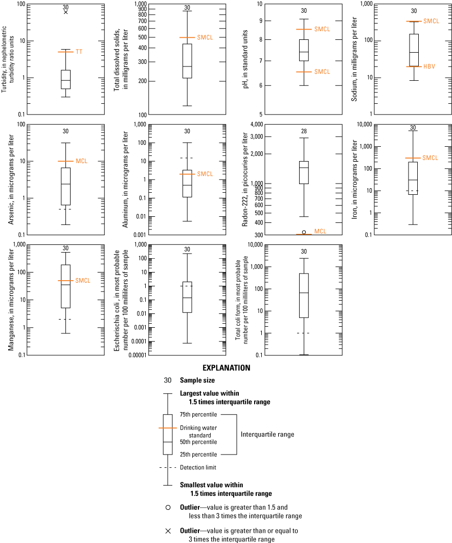
Boxplots showing distribution of concentrations of turbidity, total dissolved solids, pH, sodium, arsenic, aluminum, radon-222, iron, manganese, Escherischia coli, and total coliform, all of which exceed one or more of the drinking-water standards for 10 percent or more of the sites sampled within the wet gas dominated part of the Marcellus Shale oil and gas play in northwestern West Virginia.
Field Measurements of pH, Alkalinity, Turbidity, Specific Conductance, and Dissolved Oxygen
Of the water properties measured in the field, only pH and turbidity exceeded drinking-water standards (table 7). Turbidity exceeded the 5 nephelometric turbidity unit (NTU) EPA MCL drinking water standard in 2 of 30 (7 percent) wells sampled and exceeded the 1 NTU SWTR TT standard in 12 of 30 (40 percent) wells sampled (table 7). Turbidity is common in many wells in West Virginia and may be related to iron oxyhydroxide precipitates or sediment carried into the aquifers from the shallow soil zone due to improperly cased wells or transported to the aquifer in shallow stress relief fracture zones (Chambers and others, 2012). Many residents of northwestern West Virginia have filtration systems to remove turbidity from their well water. For this study, all samples were collected prior to any filtration or other treatment and were therefore indicative of total and dissolved constituents in the untreated water. The minimum, maximum, mean, and median turbidity levels for the 30 sites sampled were 0.3, 60, 3.21, and 0.85 NTUs, respectively (table 8).
Table 8.
Statistical summary of analytical and well-construction data for constituents analyzed in water samples from the 30 sites sampled in the wet gas dominated part of the Marcellus Shale oil and gas play in northwestern West Virginia.[Chemical data referenced in this table are available from the USGS National Water Information System database (U.S. Geological Survey, 2021) and the methane, ethane, and benzene data are available in a USGS data release (Haase and others, 2022). min, minimum value; max, maximum value; SD, standard deviation; ft, foot; bls, below land surface; mg/L, milligrams per liter; std, standard; µS/cm, microsiemens per centimeter at 25 degrees Celsius; °C, degrees Celsius; NTU, nephelometric turbidity units; <, less than; TDS, total dissolved solids; E. coli, Escherichia coli; MPN/100 mL, most probable number per 100 milliliters of sample; >, greater than; µg/L, micrograms per liter; E, number noted in scientific notation format; pCi/L, picocurie per liter; Th-230, thorium 230; Cs-137, cesium-137; mg/kg, milligram per kilogram]
The EPA SMCL drinking water standard for pH, which is a measure of whether water is acidic, alkaline, or neutral, is 6.5 to 8.5; pH values greater than 8.5 are considered alkaline water and pH values less than 6.5 are considered acidic water, both of which can be corrosive to plumbing fixtures. Corrosive water can cause trace elements and other contaminants to leach from plumbing lines and plumbing fixtures, especially those of metallic composition such as copper or galvanized steel pipes. Five of the wells sampled, (17 percent) were outside the pH SMCL range (table 7). Of those 5 sites, 4 (80 percent) were indicative of alkaline water and only 1 (20 percent) was indicative of acidic water. The minimum, maximum, mean, and median pH levels for the 30 wells sampled were 6.0, 9.1, 7.5, and 7.4 standard pH units, respectively (table 8).
Corrosivity and Potential for Galvanic Corrosion
Alkaline or acidic water can leach iron, lead, copper, zinc, and other metallic components from galvanized or copper plumbing systems. A recent USGS report computed two indices of potential corrosivity, the Langelier Saturation Index (LSI) and the potential to promote galvanic corrosion (PPGC), for groundwater across the United States, and indicated that West Virginia was among the States with a high potential for corrosive groundwater (Belitz and others, 2016).
The LSI is a measure of calcite saturation and can be used as an indicator of the potential for calcium scale to form in plumbing. The index is computed based on pH, water temperature, and concentrations of TDS, calcium, and alkalinity. The LSI was computed for all 30 wells sampled in the current study (table 9) and interpreted in the following manner. An LSI less than -0.5 is classified as potentially corrosive, an LSI is classified as indeterminate if greater than or equal -0.5 and less than or equal to 0.5, and classified as scale forming if greater than 0.5. Of the 30 wells sampled, 27 sites (90 percent) had an LSI less than -0.5 indicative of corrosive waters, 3 sites (10 percent) had LSI values in the indeterminate range, and none (0 percent) of the wells sampled had an LSI value of alkaline scale-forming water.
Table 9.
Calculated Langelier Saturation Index, chloride to sulfate mass ratio, and potential to promote galvanic corrosion rating for the 30 wells sampled in the wet-gas-dominated part of the Marcellus Shale oil and gas play in northwestern West Virginia.[ft, foot; bls, below land surface; NAVD 88, National Vertical Datum of 1988; LSI, Langelier Saturation Index; CSMR, chloride to sulfate mass ratio; PPGC, potential to promote galvanic corrosion; Cal, Calhoun County; Dod, Doddridge County; Gil, Gilmer County; Rit, Ritchie County; Roa, Roane County; Tyl, Tyler County, Wet, Wetzel County; Wir, Wirt County]
The corrosivity of water is insufficient to assess whether water from a particular well has a potential to leach trace metals from galvanized pipes and boilers or from copper pipe soldered with lead tin solder. The PPGC can be estimated from the chloride to sulfate mass ratio (CSMR). Nguyen and others (2011) developed a decision tree to help public water utilities evaluate treatment alternatives that might prevent galvanic corrosion of lead pipes and plumbing features. Three levels of concern were defined based on the CSMR and alkalinity: no concern, significant concern, and serious concern (Nguyen and others, 2011). Nguyen and others (2011) noted that if no lead is present in a system, or if partially replaced lead components exist, then the classification is “no concern.” However, for this current study, untreated groundwater was assessed and the three-tier classification system was applied without consideration of the presence or absence of lead in the raw source water or within the water distribution system to assess the PPGC for the wells sampled. The three PPGC levels for this study, which are defined based on chloride-sulfate mass ratios and the alkalinity, are classified as low, moderate, and high: if the CSMR is less than 0.2, then the PPGC is low; if the CSMR is greater than or equal to 0.2 but less than or equal to 0.5, then the PPGC is moderate; if the CSMR is greater than 0.5 and alkalinity is greater than or equal to 50, then the PPGC is moderate; and if CSMR is greater than 0.5 and alkalinity is less than 50, then the PPGC is high.
Of the 30 wells sampled, none (0 percent) had a PPGC that classified as high, 26 (87 percent) were classified as moderate, and 4 (13 percent) were classified as low. Since the PPGC classification is based partly on total alkalinity, the moderate to high levels of alkalinity present in groundwater in the study area buffer the water and reduce the potential to promote galvanic corrosion in public and residential water systems in the study area. Preliminary evaluation using graphical analysis (not presented in this report) of the computed LSI and PPGC did not indicate any potential correlation to well depth, geologic formation, or topographic setting, and thus no further analysis of data by population comparison using Wilcoxon Signed Rank Test or similar tests of statistical significance was done.
Indicator Bacteria
Both total coliform bacteria and E. coli were detected in one or more groundwater samples (tables 7, 8) at concentrations exceeding the MCL and the MCLG of zero colonies per 100 mL. Total coliforms, which are a broad class of indicator bacteria, are common in groundwater in northwestern West Virginia and were detected in 26 of the 30 sites (87 percent) sampled. The presence of total coliform bacteria is a potential indicator of surface contamination due to improperly constructed or cased wells or groundwater contamination, due to surface contaminants entering groundwater through stress-relief fractures or other direct connections to groundwater aquifers such as those caused by subsidence related to underground coal mining or solution channels and conduits in limestone. The presence of total coliform bacteria is not necessarily an indicator of potential pathogens in the water due to their common occurrence; however, they can indicate that the well may be subject to bacterial and viral pathogens. E. coli., a subset of total coliform bacteria, however, are indicative of fecal contamination of groundwater from either human or animal sources. Eleven of the 30 (37 percent) wells sampled had detections of E. coli, which may be an indicator of other related pathogens such as viruses (table 7; U.S. Environmental Protection Agency, 2019). In these cases, chlorination, ozonation, or ultraviolet (UV) light treatment may be appropriate to kill potential pathogenic microorganisms in source groundwater for residential and public supply. County Health Departments are available to assist homeowners in evaluating results of bacterial tests and for advising homeowners as to possible treatment options.
Nutrients
Nitrate and nitrite are common nutrients that can exceed drinking-water standards in agricultural areas of West Virginia, but the occurrence of nitrate and other nutrients at concentrations approaching drinking-water standards is uncommon for non-agricultural areas of the State (Chambers and others, 2012). There is little agricultural activity within the study area and only a small proportion of land is in (primarily cattle) pasture (150.6 mi2 or 5.5 percent of the study area), and therefore agricultural activities in the study area would likely only be a limited source of nutrients. Although nitrate is commonly derived from synthetic agricultural fertilizers and animal manure, nitrate can also be derived from septic system effluent in the study area.
Nitrate and nitrite concentrations in groundwater samples from the 30 wells sampled were very low and none of the concentrations of these constituents in the samples exceeded the 10 or 1 mg/L EPA MCL for either nitrate or nitrite, respectively (table 7). The maximum nitrate and nitrite concentrations were 3.79 and 0.008 mg/L, respectively. Median nitrate, nitrite, ammonia, and orthophosphate concentrations were all low, with concentrations of less than 0.040, less than 0.001, 0.08, and 0.015 mg/L, respectively (table 8). These concentrations are similar to those found in a statewide assessment of groundwater quality (Chambers and others, 2012). Only one site had a nitrate concentration greater than 1 mg/L. Of the sites with detectable concentrations of nitrate, 13 of 13 (100 percent) had detectable concentrations of total coliform bacteria and 8 of 13 (62 percent) had detectable concentrations of E. coli bacteria. Sources of the low nutrient concentrations with concurrent detectable bacteria are not known but could be related to septic effluent, feces from wildlife, connection to streams with a high fecal waste load, atmospheric deposition, or a combination of these various sources. Ammonia, which is typically only present in reduced waters in substantial concentrations, also was generally very low for the wells sampled. Of the 30 wells sampled, 23 (77 percent) contained detectable concentrations of ammonia, but the median and maximum concentrations were low—0.080 and 0.740 mg/L, respectively (table 8). None of the samples from the 30 wells exceeded the EPA 30-mg/L HBV for ammonia (table 7).
Hardness and Major Ions
Total dissolved solids, which is a measure of the concentration of dissolved constituents in a water sample and is commonly related to water hardness, exceeded the 500-mg/L EPA SMCL in 5 of 30 (17 percent) wells sampled (table 7). Water hardness is computed using the concentrations of calcium and magnesium and typically is reported in mg/L as calcium carbonate (CaCO3). Water with hardness of 0 to 60 mg/L as CaCO3 is considered soft water and 10 of the 30 wells sampled (33 percent) had soft water. Water with a hardness of 61 to 120 mg/L as CaCO3 is considered moderately hard water, and 9 of 30 (30 percent) of the wells sampled had moderately hard water. Water with hardness greater than 121 to 180 mg/L as CaCO3 is considered hard water and was found in 7 of the 30 (23 percent) wells sampled. Only 4 of the 30 (13 percent) wells sampled had hardness greater than or equal to 181 mg/L as CaCO3, which is considered very hard water. Overall, 36 percent of the wells sampled had hardness representative of hard to very hard water and 64 percent of the wells sampled had water that was considered moderately hard to soft. Soft water can make it difficult for soap to work effectively and water that is too hard can contribute to scale deposits in water heaters and plumbing lines.
Water hardness is mostly associated with higher concentrations of calcium and magnesium and is derived primarily from the dissolution of carbonate minerals, such as calcite (calcium carbonate) or dolomite (calcium magnesium carbonate), which are common components of limestone and calcareous shales. However, other non-carbonate mineral dissolution such as gypsum (calcium sulfate) and calcium or magnesium chloride salts can contribute to water hardness. Calcium, magnesium, sodium, potassium, sulfate, chloride, silica, and bicarbonate are the major ions that contribute to the TDS content of water within the study area, and the median concentrations of these constituents for the 30 wells sampled were 29.1, 4.90, 48.7, 1.22, 10.8, 10.1, 11.4, and 240 mg/L, respectively (table 8).
Sodium, chloride, fluoride, and sulfate are common constituents in groundwater within the study area, detected at various concentrations in samples from all 30 wells. These constituents can be derived from natural sources and (or) human activities. Sulfate and chloride in water can impart a salty taste at concentrations greater than 250 mg/L. Sulfate and chloride concentrations in the study area were generally low—none (0 percent) of the wells sampled contained sulfate exceeding the EPA SMCL of 250 mg/L and only 2 of 30 (7 percent) sites sampled contained chloride in excess of the 250-mg/L EPA SMCL (table 7). Sodium has an EPA HBV of 20 mg/L for individuals who are on a sodium-restricted diet for blood pressure or other health reasons (table 7). Sodium concentrations were elevated at many of the wells sampled, with 24 of 30 (80 percent) exceeding the 20 mg/L HBV (table 7). Fluoride in high concentrations can cause mottling or discoloration of teeth (U.S. Environmental Protection Agency, 2022b). The EPA SMCL for fluoride is 2.0 mg/L. Only 1 of 30 (3 percent) wells sampled contained fluoride (2.86 mg/L) greater than the SMCL (tables 7, 8).
Composition of groundwater for the wells sampled is shown in a trilinear diagram, which shows the distribution of major cations and anions for the wells sampled (fig. 8). The trilinear diagrams show that most groundwater samples within the study area can be categorized as either a calcium-magnesium bicarbonate water type (14 sites) or a sodium-potassium bicarbonate type of water (13 sites). There were two sites that have a sodium-potassium sulfate-chloride type of water and one site with a calcium-magnesium sulfate-chloride type of water. Shallow discharge of saline water has been documented at locations within the study area (Hennen, 1911), and these three sites may be affected by upwelling of deeper saline or brackish groundwater. Sources of chloride will be discussed later in this report in relation to bromide.
Metals and Trace Elements
Manganese, aluminum, and iron were detected commonly in the groundwater samples collected for this study. Manganese concentrations exceeded the 50-µg/L SMCL drinking water standard in 14 of 30 (47 percent) sites analyzed; aluminum concentrations exceeded the 2.0-µg/L SMCL drinking-water standards in 7 of 30 (23 percent) sites; and iron exceeded the 300-µg/L SMCL drinking-water standards in 5 of 30 (17 percent) sites (table 7). Two of the 30 (7 percent) wells sampled had concentrations of manganese that exceeded the 300-µg/L USGS HBSL, but none of the wells sampled exceeded the 1,600-µg/L EPA DWEL, which is based on a lifetime exposure level. There are no applicable HBSLs or DWELs for iron or aluminum in drinking water. The median, maximum, and minimum concentrations of iron for the 30 wells sampled were 31.1 and 5,150 µg/L and less than the 10-µg/L method detection limit, respectively. The median, maximum, and minimum concentrations of manganese for the 30 wells sampled were 35.2 and 527 µg/L and less than the 0.4-µg/L method detection limit, respectively. The maximum concentration of aluminum for the 30 wells sampled was 101 µg/L, but the median and minimum aluminum concentrations for wells sampled was less than the 3.0-µg/L method detection limit, respectively (table 8).
Lead concentrations in samples from the 30 wells were low and none (0 percent) of the wells sampled had lead concentrations that exceeded the EPA TT drinking water action level of 15 μg/L. The EPA MCLG for lead is 0 and 23 of 30 (77 percent) of the wells sampled contained lead at detectable concentrations (table 7). However, the maximum lead concentration detected was only 0.998 μg/L, with median and minimum concentrations of 0.077 μg/L and less than the 0.020-μg/L method detection limit, respectively (table 8).
Arsenic is a potential contaminant of concern for health within the study area; 7 of 30 (23 percent) wells sampled had arsenic concentrations exceeding the 10-µg/L EPA MCL health-based drinking water standard (table 7). The EPA MCLG for arsenic is 0 µg/L and 29 of 30 (table 7) wells sampled contained detectable concentrations of arsenic. The maximum, median, and minimum arsenic concentrations for the wells sampled were 31.4 and 2.40 µg/L and less than the 0.19-µg/L method detection limit, respectively (table 8).
Mercury was detected only at 1 of 30 (3 percent) wells sampled, at a concentration of 0.008 µg/L, exceeding the EPA MCLG of 0 for mercury but did not exceed either the EPA MCL or DWEL (tables 7, 8). In comparison, none of the 30 wells sampled had antimony, barium, beryllium, cadmium, chromium, copper, selenium, silver, or zinc concentrations exceeding the EPA MCLs, MCLGs, SMCLs, DWELs, nor molybdenum or nickel concentrations exceeding EPA DWELs or USGS HBSLs (table 7). Median concentrations of barium and zinc were 222 and 4.70 µg/L, respectively, and median concentrations of antimony, beryllium, cadmium, chromium, copper, selenium, and silver were all low, with median concentrations for the 30 wells sampled less than the method detection levels of 0.06, 0.01, 0.03, 0.5, 0.4, 0.05, and 1.0 µg/L, respectively (table 8). Except for barium, median concentrations of trace metal constituents were typically at or below the method detection limits.
Dissolved Hydrocarbon Gases
The highest concentrations of any of the dissolved hydrocarbon gases measured were for methane, followed by ethane, ethene, and propane, in decreasing concentrations, and were detected in samples from all 30 wells sampled (tables 7, 8). Methane and other dissolved hydrocarbons are potentially explosive combustible gases that are commonly related to the production of oil and gas, which is a dominant land use in the study area. Therefore, this study helps to assess the potential for these gases to be present in groundwater in the study area. There are no EPA drinking-water standards for methane gas or the other measured dissolved hydrocarbons except for benzene. The EPA MCL and MCLG goals for benzene are 5.0 and 0.0 mg/L, respectively. Benzene was detected at 11 of 30 (37 percent) wells sampled (table 8) and none (0 percent) of the sites had concentrations of benzene in excess of the EPA MCL drinking water standard (table 7). Concentrations of most dissolved hydrocarbons, except methane, were very low, with samples typically having a total C2 to C6 hydrocarbon concentration on the order of 1.0 × 10⁻⁴ milligrams per kilogram (mg/kg), corresponding to partial pressures in the range of air-water equilibrium; the maximum benzene concentration was only 9.84 × 10⁻⁶ mg/kg (table 8). At standard temperature and pressure, mg/kg and mg/L are equivalent for water with a density of 1.0, such as fresh groundwater.
The OSMRE published LOC for methane in groundwater is 10 mg/L and the IAL at which mitigation of a gas is recommended is 28 mg/L (Eltschlager and others, 2001). Only 1 of 30 (3 percent) wells sampled for methane gas had a concentration (17.9 mg/kg) exceeding the 10-mg/L OSMRE LOC and none exceeded the 28-mg/L IAL (table 7). Median, minimum, and maximum concentrations of methane gas for the 30 wells sampled were 0.042, 3.51 × 10⁻⁵, and 17.9 mg/kg, respectively (table 8).
Radioactive Constituents
Radon-222, radium-224, radium-226, radium-228, uranium, uranium-234, uranium-235, uranium-238, and gross-alpha and gross-beta radioactivity were analyzed and detected in water from many of the 30 wells sampled (tables 7, 8). These constituents are commonly associated with organic-rich dark shales such as the Marcellus Shale. A statewide assessment of groundwater quality in West Virginia (Chambers and others, 2012) indicated that although radon-222 concentrations did not commonly exceed the EPA proposed MCL of 300 pCi/L or AMCL of 4,000 pCi/L for radon in drinking water, there were select areas, primarily in the western part of the State coincident with the study area for this investigation, that had the potential for radon gas concentrations in drinking water in excess of the proposed MCL. Though all 30 wells were sampled for these radioactive constituents, two radon-222 samples were lost in shipment, and therefore discussion for radon-222 is based on 28 samples instead of 30 samples for the other radionuclides. Samples from all 28 wells (100 percent) exceeded the EPA proposed MCL of 300 pCi/L for radon-222, but none exceeded the 4,000-pCi/L AMCL (tables 7, 8), which is applicable to public drinking water systems that have adopted radon mitigation programs. Wells with radon gas concentrations exceeding the 300-pCi/L proposed MCL in groundwater have the potential for airborne concentrations of radon-222 to exceed the EPA 4-pCi/L indoor air standard. Inhalation of radon can cause lung cancer and the 4-pCi/L indoor air standard is based on an inhalation standard (Otton, 1992). Therefore, homeowners whose wells have dissolved radon-222 gas concentrations exceeding 300 pCi/L may be advised to test their indoor air concentrations. The mean radon-222 concentration was 1,461 pCi/L, the median was 1,450 pCi/L, and the maximum and minimum radon-222 concentrations were 2,910 and 320 pCi/L, respectively (table 8).
None of the wells sampled had uranium concentrations exceeding the 30-µg/L EPA MCL drinking water standard (table 7). The EPA MCLG for uranium is 0 µg/L and 18 of the 30 (60 percent) wells sampled had detectable concentrations of uranium (tables 7, 8). The maximum uranium concentration for wells sampled was 2.63 µg/L, the mean concentration was 0.241 µg/L, but the median concentration was much less at 0.072 µg/L (table 8).
There are no applicable EPA drinking-water standards for uranium-234, uranium-235, uranium-238, or radium-224. There is an EPA MCL for combined radium-226 and radium-228 of 5 µg/L and an EPA MCLG of 0.0 µg/L for combined radium-226 and radium-228. For the 30 wells sampled, none exceeded the 5-µg/L EPA MCL, but 29 of the 30 wells sampled (97 percent) had detectable concentrations of combined radium-226 and radium-228 (table 7). However, mean and median concentrations of radium-226 and radium-228 were both low and in most cases just above the method detection limits. Mean radium-226 and radium-228 concentrations were 0.358 and 0.520 µg/L, respectively, and median radium-226 and radium-228 concentrations were 0.150 and 0.450 µg/L, respectively (table 8).
Relation to Geologic Formation
The composition of the bedrock in which the water wells are completed can affect the quality of groundwater derived from the rural residential wells sampled for this study. There is substantial variability with respect to lithologic composition between the various geologic formations (fig. 8A, table 10) and even within individual strata that comprise the geologic formations (figs. 9, 10). There were statistically significant differences with respect to calcium, magnesium, potassium, silica, and turbidity (table 11). Calcium, magnesium, potassium, silica, and turbidity concentrations were statistically significantly higher in the Dunkard Group than in the Conemaugh Group or Allegheny Formation (tables 10, 11). Although not statistically significant, median sodium concentrations are highest in wells sampled in the Monongahela Formation (fig. 11). The surface geology does not allow for assessing from which specific strata (sandstone, limestone, siltstone, shale, or coal) a particular well may be deriving water. In fact, wells may obtain water from multiple intervals and therefore the following discussion is based on the major geologic groups and formations within the study area (Conemaugh Group, Monongahela Formation, or Dunkard Group).
Table 10.
Statistical summary of the mean, median, and maximum values for select constituents analyzed in water samples from the 30 sites sampled in the wet gas dominated part of the Marcellus Shale oil and gas play in northwestern West Virginia by geologic group or formation.[Data referenced in this table are available from the USGS National Water Information System (NWIS) database (U.S. Geological Survey, 2021); NA, not applicable; ft, foot; bls, below land surface; mg/L, milligrams per liter; std, standard; µS/cm, microsiemens per centimeter at 25 degrees Celsius; NTU, nephelometric turbidity units; TDS, total dissolved solids; − + NO2, nitrate plus nitrite; <, less than; E. coli, Escherichia coli; MPN/100 mL, most probable number per 100 milliliters of sample; >, greater than; µg/L, micrograms per liter; pCi/L, picocuries per liter; Th-230, thorium 230; Cs-137, cesium-137; mg/kg, milligram per kilogram]
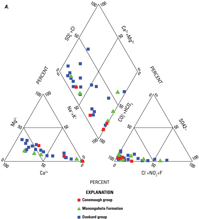
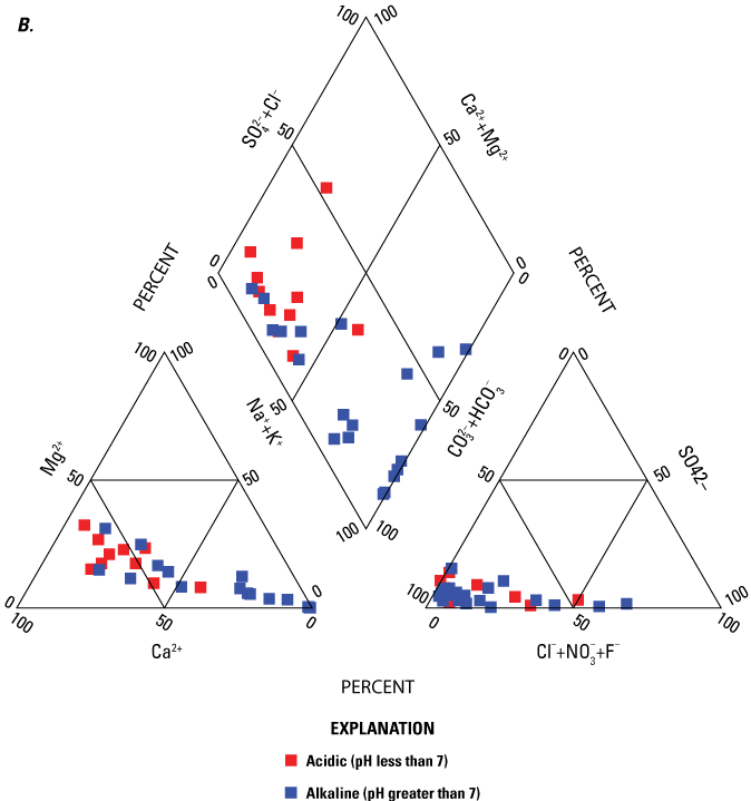
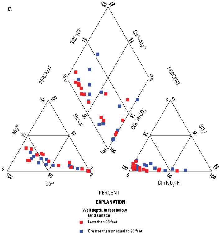
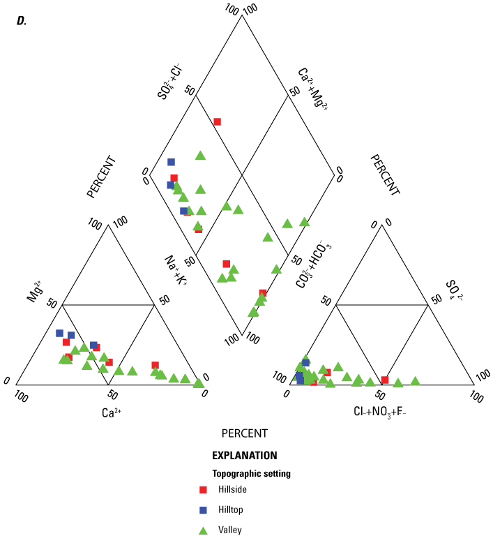
Trilinear diagrams showing the magnesium, sulfate, calcium, bicarbonate, sulfate, chloride, nitrate, fluoride, sodium, and potassium ion composition in groundwater samples for 30 wells in the wet-gas-dominated part of the Marcellus Shale oil and gas play in northwestern, West Virginia by A, geologic formation or group, B, ph, C, depth of well, and D, topographic setting.
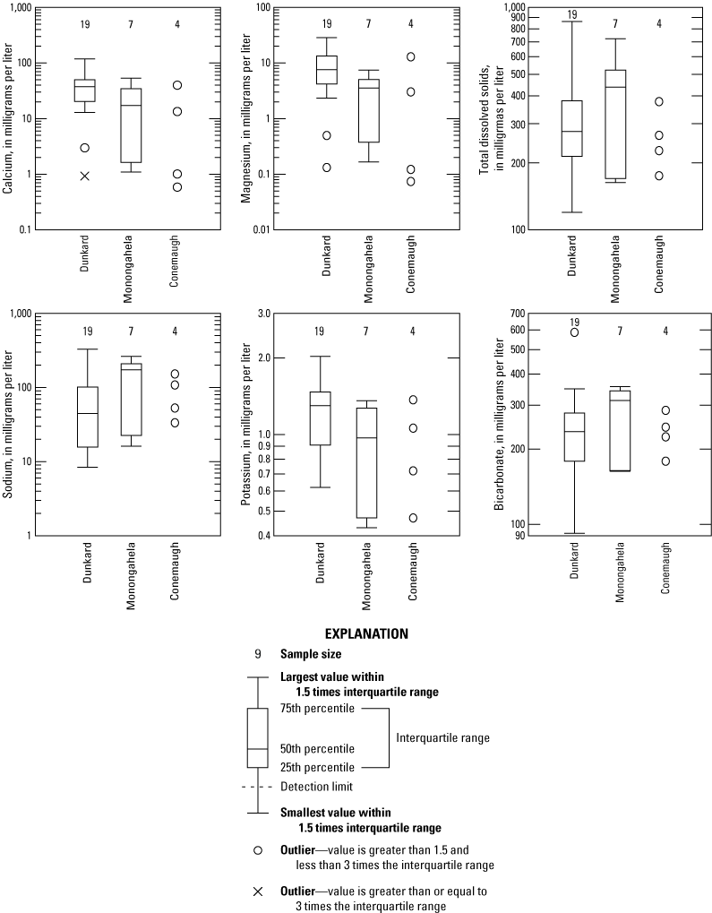
Boxplots showing distribution of calcium, magnesium, total dissolved solids, sodium, potassium, and bicarbonate in groundwater samples for 30 wells in the wet gas dominated part of the Marcellus Shale oil and gas play in northwestern West Virginia grouped by geologic formation or group.
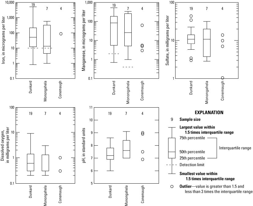
Boxplots showing distribution of iron, manganese, sulfate, dissolved oxygen, and pH in groundwater samples for 30 sites in the wet gas dominated part of the Marcellus Shale oil and gas play in northwestern West Virginia grouped by geologic formation or group.
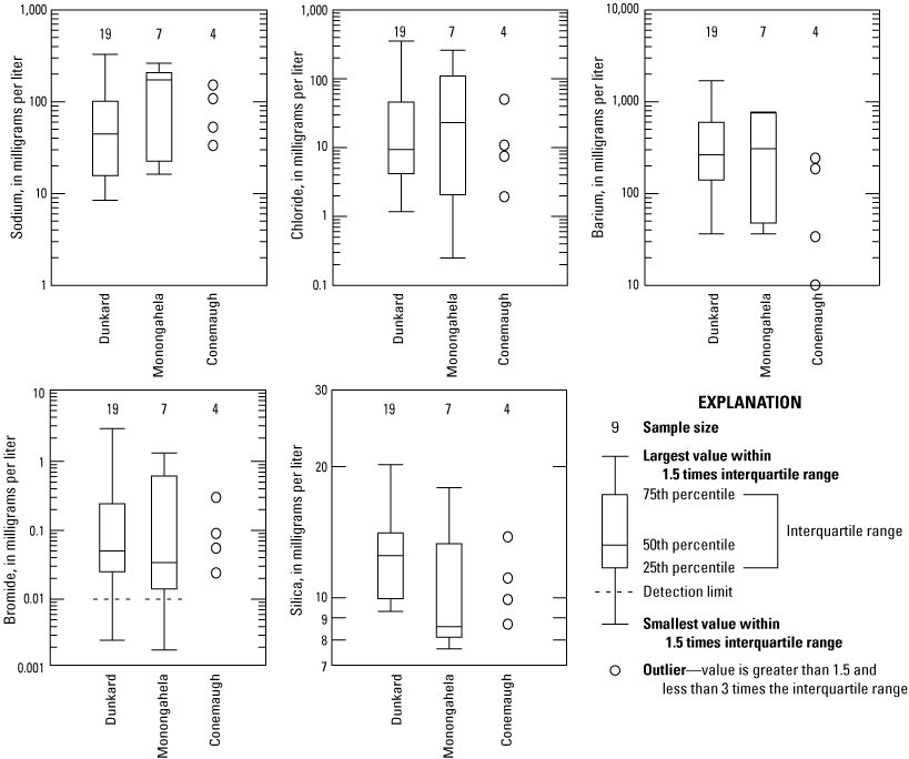
Boxplots showing distribution of sodium, chloride, barium, bromide, and silica in groundwater samples for 30 wells in the wet gas dominated part of the Marcellus Shale oil and gas play in northwestern West Virginia grouped by geologic formation or group.
Table 11.
Tests of statistical significance using the Wilcoxon Signed Rank Test with respect to geologic groups or formations, topographic setting (upland sites compared to valley sites), well depth (< 95 or ≥ 95 feet in depth), number of pre-1930 oil and gas wells within 1,000 m, number of Marcellus Shale oil and gas wells within 1,000 m, and total number of oil and gas wells within 500 m of the 30 residential wells sampled in the wet gas dominated part of the Marcellus Shale oil and gas play in northwestern West Virginia.[<, less than; ft, foot; ≥, greater than or equal to; ≤, less than or equal to; m, meters; n, sample size; E. coli, Escherichia coli; TDS, total dissolved solids; N, nitrogen]
Major Ions, Total Dissolved Solids, and Turbidity
An examination of the maximum, median, and mean concentrations for select constituents related to the various geologic groups or formations (table 10) indicate that there is variability in chemical constituent concentrations. The most significant trend in the statistical data with respect to geologic formation or group was to water hardness, calcium, magnesium, potassium, carbon dioxide, turbidity, dissolved oxygen, silica, nitrate, aluminum, iron, lead, manganese, strontium, selenium, uranium-234, uranium-238, radium-238, gross beta radiation, and the indicator bacteria total coliform and E. coli, which were all greater in water samples from wells completed in the Dunkard Group than in water samples from wells completed in either the Monongahela Formation or Conemaugh Group. Mean and median concentrations of specific conductance, alkalinity, bicarbonate, total dissolved solids, sodium, chloride, fluoride, molybdenum, gross alpha radiation, radium-224, radon-222, and uranium-235 were greater in water samples from wells sampled in the Monongahela Formation than from the Conemaugh or Dunkard Groups. Mean and median pH and concentrations of orthophosphate, radium-228, and ethane were greater in water sampled from wells in the Conemaugh Group than from wells sampled in either the Dunkard Group or the Monongahela Formation.
A trilinear diagram comparing major ion composition for the Conemaugh Group, Monongahela Formation, and the Dunkard Group (fig. 8A) does not show a substantial difference in water type for the various geologic groups or formations. This is not unexpected, as the trilinear diagram also shows variability in the composition of the major cations and anions comprising the waters sampled for the two dominant geologic groupings, and there are obvious differences in the overall composition as evidenced by the mean, median, and maximum cation and anion values (table 10). The dominant type of water for sites in all the geologic formations or groups varied between a calcium-magnesium bicarbonate water type (14 sites) to a sodium-potassium bicarbonate water type (13 sites), with additional sites being of a sodium-potassium sulfate-chloride water type (2 sites) or a calcium-magnesium sulfate-chloride water type (1 site).
A boxplot of the major cations that typically represent the majority of TDS in a water sample (fig. 9) shows higher median concentrations of calcium, magnesium, and potassium for water from wells sampled in the Dunkard Group than for wells completed in the Conemaugh Group or Monongahela Formation. Sodium concentrations were higher for wells sampled in the Conemaugh Group or Monongahela Formation than in the Dunkard Group.
There were statistically significant differences in concentrations of calcium, magnesium, potassium, silica, and turbidity for Dunkard Group wells compared with the combined data for the Conemaugh Group and Monongahela Formation. Results of the Wilcoxon Signed Rank Test of statistical comparison of populations (table 11) and statistical summaries of constituents by geologic group or formation (table 10) shows that the overall TDS, calcium, magnesium, potassium, and hardness concentrations are higher for wells sampled in the Dunkard Group than for wells sampled in the Conemaugh Group or Monongahela Formation (fig. 9). Concentrations of sodium are highest in groundwater sampled from the Conemaugh Group and Monongahela Formation (fig. 9).
Median concentrations of calcium, magnesium, potassium, silica and turbidity for wells sampled in the Dunkard Group (table 10) were 37.6, 7.55, 1.30, and 12.5 mg/L and 1.2 NTU, respectively, while median concentrations for the same constituents for wells sampled in the Monongahela Formation were 17.2, 3.55, 0.97, and 8.59 mg/L and 0.5 NTU, respectively, and for the wells sampled in the Conemaugh Group were 7.21, 1.57, 0.89, and 10.5 mg/L and 0.4 NTU, respectively. Further assessment of the geochemical processes that may be responsible for the differences in these and other chemical constituent concentrations and field measured parameters of dissolved oxygen, pH, specific conductance, and well depth will be discussed in the Geochemistry section of this report.
Iron, Manganese, pH, and Sulfate
The more problematic chemical constituents with respect to aesthetic concerns in groundwater in West Virginia are typically iron, manganese, sulfate, and pH (Chambers and others, 2012). Iron and manganese are not depicted in the trilinear diagrams comparing geologic formations (figs. 8A, 9) because they are not typically dominant ions with respect to the overall TDS of groundwater. Alkaline groundwater can induce corrosion of galvanized and copper water lines resulting in boiler scale deposits and imparting a poor taste to the water.
Boxplots of iron, manganese, sulfate, dissolved oxygen, and pH show that there are differences in the median concentrations for the sites in the various geologic formations (fig. 10) and are likely related to mineral composition of the bedrock within the various geologic groups or formations and to redox or other geochemical processes, as shown by higher median iron and manganese concentrations and lower mean pH in wells sampled from the Dunkard Group as compared to wells sampled in the Conemaugh Group and Monongahela Formation (fig. 10, table 10).
There are also differences in constituent concentrations between waters with pH characteristic of alkaline (pH greater than 7) and acidic (pH less than 7) waters (fig. 12A, B). Acidic waters consistently have higher concentrations of calcium, magnesium, potassium, and zinc. Alkaline (or basic) waters have consistently higher concentrations of bicarbonate, sodium, fluoride, and molybdenum. These relations partly reflect relative solubilities of the constituents under various pH conditions.
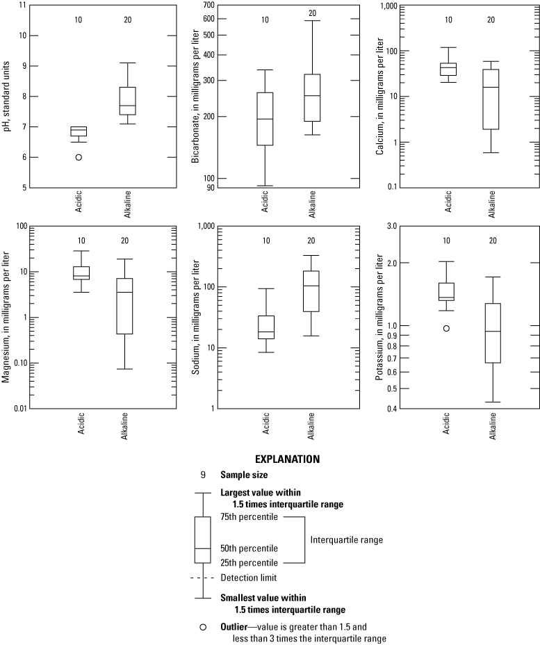
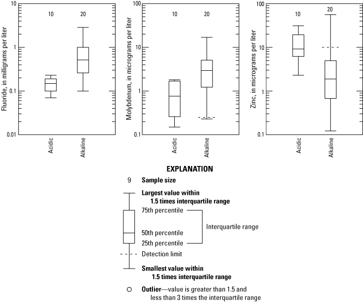
Boxplots of pH, bicarbonate, calcium, magnesium, sodium, potassium, fluoride, molybdenum, and zinc in groundwater analyzed for the 30 sites sampled in the wet gas dominated part of the Marcellus Shale oil and gas play in northwestern West Virginia with respect to pH.
A trilinear diagram (fig. 8B) showing the distribution of major cations and anions classified with respect to pH indicates that geochemical processes exert strong influence on the distribution of dominant cations and anions, with waters of acidic composition being primarily a calcium-magnesium bicarbonate type of water and waters of an alkaline composition being primarily a sodium-potassium bicarbonate water type.
Results of the Wilcoxon Signed Rank Tests of statistical significance did not indicate a statistically significant difference in concentrations of iron, manganese, sulfate, or pH when comparing samples collected from wells in the Dunkard Group to samples collected from wells completed in the Conemaugh Group and Monongahela Formation, although the p value of statistical significance for pH (0.092) was close to the p value of 0.05 indicating statistical significance at a confidence interval of 95 percent (table 11). However, the lack of a trend with respect to geologic formation or group could have been due to limited data for the Conemaugh Group, which was combined for statistical analysis with data for the Monongahela Group.
Concentrations of iron, manganese, and dissolved oxygen were highest, and pH was lowest, in wells sampled in the Dunkard Group with median concentrations of 51.7 µg/L, 84.1 µg/L, 0.60 mg/L, and 7.2 standard units, respectively (table 10). Median concentrations of iron, manganese, dissolved oxygen, and median pH values for wells sampled in the Conemaugh Group were 10.0 µg/L, 5.28 µg/L, 0.30 mg/L, and 8.2 standard units, respectively (table 10). Median concentrations of iron, manganese, dissolved oxygen, and median pH values for sites sampled in the Monongahela Formation were 13.3 µg/L, 25.8 µg/L, 0.30 mg/L, and 7.6 standard units, respectively (table 10).
Median pH for water sampled from the various geologic formations and groups were all alkaline. Such high pH values are not common in groundwater in West Virginia (Chambers and others, 2012). Of special note was the median pH value of 8.2 for wells sampled in the Conemaugh Group. Limestones within the Conemaugh Group, as previously discussed in the Hydrogeologic Setting and Groundwater Flow section of this report, are primarily of marine deposition (U.S. Geological Survey and Association of American State Geologists, 2020a), which may indicate a higher solubility than the non-marine limestones, which are characteristic of the Monongahela Formation and the Dunkard Group.
Median sulfate concentrations (10.8 mg/L) are identical for wells sampled in the Monongahela Formation and Dunkard Group as compared to wells sampled in the Conemaugh Group, which has a median sulfate concentration of 8.45 mg/L. Overall sulfate concentrations for the various geologic groups and formations are all very low, with maximum concentrations for the Conemaugh Group, Monongahela Formation, and Dunkard Group of 13.9, 31.7, and 43.9 mg/L, respectively.
Constituents of Brines and Sandstones
A boxplot of the distribution of sodium, chloride, barium, and bromide (fig. 11) shows the distribution of constituents that are potentially indicative of a brine signature, although sodium and chloride can be introduced to groundwater from human activities such as septic systems and use of road salt. Generally, there is little variation with respect to concentrations of barium, bromide, and chloride (fig. 11) in relation to geologic formation and these constituents did not indicate any statistically significant relations with respect to geologic formation or topography (table 11). Water sampled from wells in the Dunkard Group had higher mean and median concentrations of silica than water from wells in the Conemaugh Group and Monongahela Formation (fig. 11, table 10). Water sampled from wells in the Conemaugh Group and Monongahela Formation had higher mean and median concentrations of sodium than water sampled from wells in the Dunkard Group (fig. 11, table 10), although there were no statistically significant differences in the concentrations of either silica or sodium between the various geologic formations or groups.
Median barium, bromide, and chloride concentrations for wells sampled in the Dunkard Group were 264 µg/L, 0.050 mg/L, and 9.36 mg/L, respectively. Median barium, bromide, and chloride concentrations for wells sampled in the Conemaugh Group were 110 µg/L, 0.073 mg/L, and 9.20 mg/L, respectively. Median barium, bromide, and chloride concentrations for wells sampled in the Monongahela Formation were 308 µg/L, 0.034 mg/L, and 23.0 mg/L, respectively. The source of higher barium and chloride concentrations in the Monongahela Formation is not known, but both constituents are commonly found in deeper saline brines. In addition to sulfate minerals, such as barite and barite-celestite solid solutions, barium may be a trace component in carbonate minerals or adsorbed by manganese oxides (Hanshaw and Back, 1979). Regardless of the potential source, wells sampled in the Monongahela Formation had higher median barium and chloride concentrations than wells sampled in the Dunkard or Conemaugh Groups.
Conversely, silica concentrations were highest in wells sampled in the Dunkard Group with a median concentration of 12.5 mg/L, as compared to wells sampled in the Monongahela Formation (median concentration of 8.59 mg/L) or Conemaugh Group (median concentration of 10.9 mg/L). Silicon is second only to oxygen in abundance within the Earth’s crust (Hem, 1992), and is commonly reported as silica in the form silicon oxide (SiO2). Silica is therefore common in many silicate oxide and hydroxide minerals such as quartz, kaolinite, potassium feldspars, beryl, and forsterite (Hem, 1992). Quartz and other silicate minerals are commonly found in high proportions in sandstone.
Radioactive Constituents
Boxplots of the uranium and radon-222 concentrations (fig. 13) and summary statistics showed little differences in the distribution of these constituents and other radionuclides (table 10) among the three geologic formations or groups. There were no statistically significant differences in radon-222, radium-226, or uranium between any of the geologic formations, as determined by the Wilcoxon Signed Rank Test.

Boxplots showing distribution of uranium and radon-222 concentrations in groundwater samples from 30 wells in the wet gas dominated part of the Marcellus Shale oil and gas play in northwestern West Virginia grouped by geologic formation or group.
A previous statewide study of groundwater quality in West Virginia (Chambers and others, 2012) showed that radon-222 concentrations were present in higher concentrations in younger Carboniferous units such as those in the study area—the Monongahela Formation and Conemaugh and Dunkard Groups—than in older Carboniferous units of southern West Virginia. Generally, the proportion of shale, siltstone, and mudstone varies with geologic age, with the younger Carboniferous geologic groups and formations composed of a higher proportion of dark shales than older Carboniferous geologic formations such as the Pocahontas and New River Formations, which have a higher proportion of sandstone. Radon-222 is commonly derived from uranium-bearing dark shales (Otton, 1992) such as are found in the study area within rocks of the Dunkard and Conemaugh Groups, the Monongahela Formation, and within the deeper Marcellus Shale, which is a natural gas reservoir of dark shale containing methane, ethane, and other dissolved hydrocarbons. It is likely that the radon-222 in the water samples is derived from the geologic sequences with a higher proportion of dark shales. However, there were not sufficient data collected for this study to fully assess the source of the radon-222, which often is found in concentrations exceeding the proposed 300-pCi/L MCL drinking water standard for all rural residential wells sampled for this study. Additional discussion of radionuclides and dissolved hydrocarbons will be presented in the Dissolved Hydrocarbon Gases and Geochemistry sections of this report.
Relation to Topographic Setting
A trilinear plot (fig. 8D) differentiating the wells sampled based on topographic position, either upland (hillside and hilltop) or lowland (valley), showed greater variability in major ion content and type of water for hillside and valley wells than for hilltop wells. Three hilltop wells have a calcium-magnesium bicarbonate water type signature, whereas hillside and valley wells varied from a calcium-magnesium bicarbonate water type to a sodium-potassium bicarbonate water type. Due to similar chemistry and a small number of hilltop (3 sites) and hillside (6 sites) wells, data for these sites were combined for statistical analysis and hereafter referred to as upland wells.
Although the majority of wells sampled were located in valley settings (21 sites) and only 9 sites were located on hilltops or hillsides (upland wells), there was a statistically significant difference in concentrations of several chemical constituents with respect to topographic setting when comparing samples from valley wells to samples from upland (hilltop and hillside) wells (table 11). There were statistically significant differences in valley and upland wells, with higher concentrations of manganese, radon-222, molybdenum, ammonia, methane, and ethane in samples from valley wells and higher concentrations of total coliform bacteria, calcium, magnesium, nitrate, uranium, copper, manganese, and selenium in samples from upland wells. The mean, median, and maximum values for constituents by topographic setting (table 12) show samples from upland wells appear to have higher dissolved oxygen concentrations than samples from valley wells, a finding supported by the nearly statistically significant Wilcoxon Signed Rank Test difference (p of 0.057) for dissolved oxygen between the two groups (table 11).
Examination of boxplots of constituents for upland and valley wells (fig. 14A, B) show that concentrations of dissolved oxygen, calcium, magnesium, nitrate, uranium, and copper were greater in upland wells compared to valley wells; ammonia, radon-222, manganese, and molybdenum were greater in valley wells as compared to upland wells. As was evident for chemical constituent concentrations for deep and shallow wells, the primary process likely responsible for the differences in groundwater quality, with the exception of total coliform bacteria, between upland and valley wells are redox processes. Redox and other geochemical processes affecting groundwater quality within the study area will be discussed more fully in the Geochemistry section of this report.
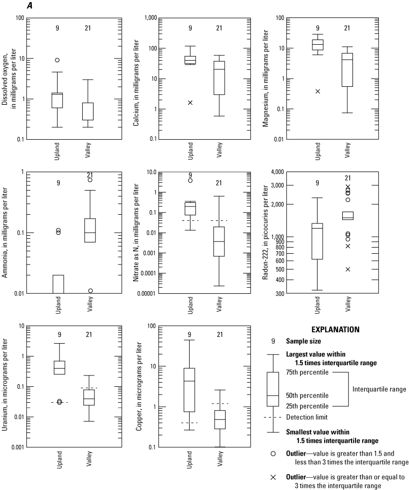
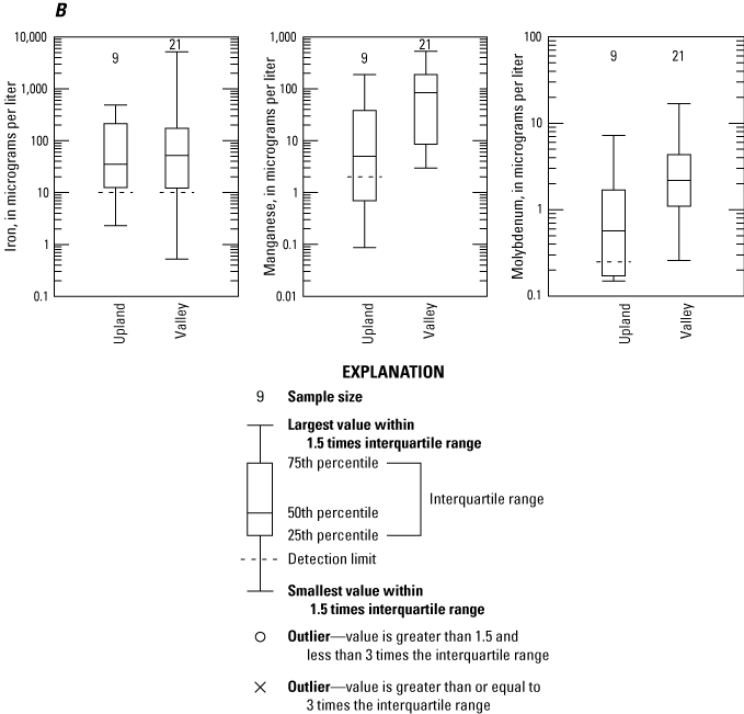
Boxplots of dissolved oxygen, calcium, magnesium, ammonia, nitrate as N, radon-222, uranium, copper, iron, manganese, and molybdenum in groundwater analyzed for the 30 wells sampled in the wet gas dominated part of the Marcellus Shale oil and gas play in northwestern West Virginia with respect to topographic setting.
Median concentrations of dissolved oxygen, calcium, magnesium, nitrate, uranium, copper, and total coliform bacteria for upland wells were 1.3 mg/L, 40.1 mg/L, 13.3 mg/L, 0.199 mg/L, 0.397 µg/L, 4.30 µg/L, and 200 colonies per 100 mL of sample, respectively, and valley wells had median concentrations of 0.3 mg/L, 20.4 mg/L, 4.17 mg/L, less than the 0.040-mg/L method detection limit, 0.060 µg/L, 0.800 µg/L, and 12 colonies per 100 mL of sample, respectively (table 12). Median concentrations of ammonia, radon-222, iron, manganese, and molybdenum for uplands wells were less than the 0.010-mg/L method detection limit, 1,200 pCi/L, 10.0 µg/L, 5.00 µg/L, and 0.571 µg/L, respectively, and median concentrations of the same constituents for valley wells were 0.100 mg/L, 1,560 pCi/L, 51.7 µg/L, 84.1 µg/L and 2.18 µg/L, respectively (table 12).
Table 12.
Statistical summary of median, mean, and maximum analytical data for select constituents analyzed in water samples from the 30 sites sampled in the wet gas dominated part of the Marcellus Shale oil and gas play in northwestern West Virginia segregated by topography.[Data referenced in this table are available from the USGS National Water Information System (NWIS) database (U.S. Geological Survey, 2021). Upland, consists of hilltop and hillside wells; NA, not applicable; ft, foot; bls, below land surface; mg/L, milligrams per liter; std, standard; µS/cm, microsiemens per centimeter at 25 degrees Celsius; NTU, nephelometric turbidity units; <, less than; TDS, total dissolved solids; NO3 + NO2, nitrate plus nitrite; E. coli, Escherichia coli; MPN/100 mL, most probable number per 100 milliliters of sample; >, greater than; µg/L, micrograms per liter; pCi/L, picocuries per Liter; Th-230, thorium 230; Cs-137, cesium-137; mg/kg, milligrams per kilogram]
Relation to Well Depth
As discussed in the previous section, geology and topographic position can have an effect on the chemical composition of the groundwater sampled, but well depth also can be a factor. The dissolved oxygen content of shallow groundwater is typically higher because of near surface processes. For this study, well depths were grouped into two bins, one bin for wells less than 95 ft in depth and a second bin for wells greater than or equal to 95 ft in depth. These groupings were based on natural break points in the data and each bin had a sample size of 15. Unfortunately, the distribution of wells available for sampling were often older wells and information on the casing length and whether the wells were grouted adequately was not available for analysis. Therefore, this discussion is solely related to the chemical constituents commonly affected by redox processes, which are contingent on the dissolved oxygen content, or lack thereof, in the wells and aquifers sampled.
The depth of wells also can affect groundwater quality, as deeper wells typically contain lower dissolved oxygen levels than shallower wells or wells with short casings. Dissolved oxygen, or the lack thereof, is a primary factor controlling redox processes in groundwater. In this study, shallower wells (less than 95 ft deep) had slightly higher dissolved oxygen, iron, manganese, radon-222, and ammonia concentrations than deeper wells, which had slightly higher concentrations of calcium, magnesium, bicarbonate, and uranium (fig. 15A, B, table 13,). Median (50th percentile) concentrations of dissolved oxygen, iron, manganese, radon-222 and ammonia for shallow wells were 0.6 mg/L, 66.6 µg/L, 62.7 µg/l, 1,615 pCi/L, and 0.120 mg/L, respectively, whereas deeper wells had lower median concentrations of dissolved oxygen, iron, manganese, radon-222 and ammonia of 0.4 mg/L, 12.2 µg/L, 6.3 µg/l, 1,075 pCi/L, and 0.070 mg/L, respectively (table 13). Median concentrations of calcium, magnesium, bicarbonate, and uranium for shallow wells were 20.4, 3.55, 185 mg/L, and less than 0.033 µg/L, respectively, whereas deeper wells had slightly higher median concentrations of calcium, magnesium, bicarbonate, and uranium of 39.9, 7.43, 262 mg/L, and less than 0.166 µg/L, respectively (table 13).
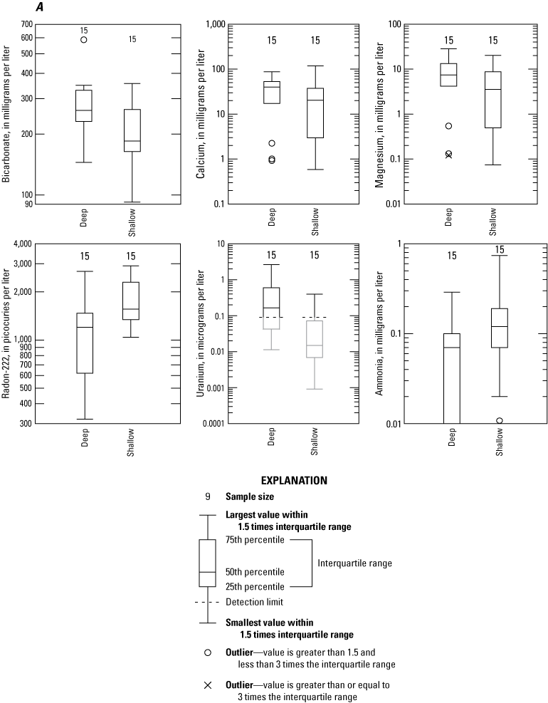
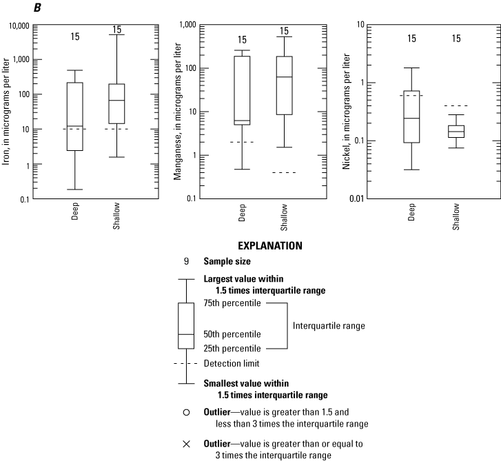
Boxplot showing variability in bicarbonate, calcium, magnesium, radon-222, uranium, ammonia, iron, manganese, and nickel in groundwater water analyzed for the 30 wells sampled in the wet gas dominated part of the Marcellus Shale oil and gas play in northwestern West Virginia with respect to well depth.
Table 13.
Statistical summary of median, mean, and maximum analytical data for select constituents analyzed in water samples from the 30 sites sampled in the wet-gas-dominated part of the Marcellus Shale oil and gas play in northwestern West Virginia segregated by well depth.[Data referenced in this table are available from the USGS National Water Information System (NWIS) database (U.S. Geological Survey, 2021). <, less than; ft, foot; ≥, greater than or equal to; NA, not applicable; bls, below land surface; mg/L, milligrams per liter; std, standard; μS/cm, microsiemens per centimeter at 25 degrees Celsius; NTU, nephelometric turbidity ratio units; NO3 + NO2, nitrate plus nitrite; E. coli, Escherichia coli; MPN/100 mL, most probable number per 100 milliliters of sample; μg/L, microgram per liter; >, greater than; pCi/L, picocuries per Liter; Th-230, thorium; Cs-137, cesium-137; E, number noted in scientific notation format; mg/kg, milligrams per kilogram]
Examination of the trilinear diagram of major ion content of the groundwater samples collected for the study did not show any obvious trends in overall types of groundwater with respect to well depth (fig. 8C) as there was variability in major ion content and water type for both shallow and deep wells. Water type generally varied from a calcium-magnesium bicarbonate type of water to a sodium-potassium bicarbonate type of water.
Wilcoxon Signed Rank Tests, computed to assess whether there were statistically significant differences in populations (table 11), confirmed statistically significant differences between deeper wells (greater than or equal to 95 ft in depth) and shallower wells (less than 95 ft in depth) for ammonia, radon-222, uranium, nickel, and bicarbonate similar to what is shown in the boxplots for these constituents grouped by depth of well (fig. 15A, B).
The primary process likely responsible for the differences in groundwater quality between deeper and shallower wells are redox processes. Redox and other geochemical processes affecting groundwater quality within the study area will be discussed more fully in the Geochemistry section of this report.
Relation to Density of Oil and Gas Wells
One primary objective of the study was to assess the water-quality data for the wells sampled with respect to the number of nearby oil and gas production wells. Processes associated with the drilling, production, maintenance, and upgrade of oil and gas wells have been postulated to possibly affect groundwater quality within the study area. There are also many older oil and gas wells within the study area that are no longer in production and have been abandoned, as well as other wells drilled prior to 1930 that were not regulated and did not require a permit and therefore may have a higher potential for failed or failing well casings. The effect, or lack thereof, of current Marcellus Shale horizontal production wells, current or legacy traditional vertical wells, and older, pre-1930, vertical wells is assessed within this report. Statistical analysis was conducted using the Wilcoxon Signed Ranks Test for the three different populations of oil and gas wells. The oil and gas wells’ spatial distributions were separated into two classes of lower and higher density for each of the three populations to assess whether there were any statistically significant differences among populations with respect to the constituents sampled for this study and land use (table 11). The first population—active oil and gas wells—was classified in two classes for multivariate statistical analysis with respect to the number of Marcellus Shale oil and gas wells (n) within 1,000 m of the rural residential wells sampled, with classes of n equal to zero (n equals 0) or n greater than or equal to 1 (n ≥ 1). The second population—older, pre-1930, oil and gas wells—was within a 1,000-m radius of the residential wells sampled, with classes of n (number of pre-1930 wells) less than (<) 3 and n ≥ 4. The third population—all oil and gas wells, regardless of type or date drilled—was within a 500-m radius of the rural residential wells sampled for the study, with classes of n (number of all oil and gas wells) ≤ 4 and n ≥ 5. The classes were determined by parsing the data into roughly equivalent numbers of observations based on natural breaks in the distribution of the data.
There were no statistically significant differences in the distribution of older, pre-1930, oil and gas wells or Marcellus Shale wells for any of the chemical constituents analyzed for the study when comparing lower and higher density of oil and gas wells within a 1,000-m radius of a sampled residential water wells (table 11). There was, however, a statistically significant difference in radium-226, barium, and ethane concentrations with respect to the density of oil and gas wells within a 500-m radius around the residential wells sampled for the study, with residential wells sampled that had four or fewer oil and gas wells surrounding the wells sampled having statistically lower concentrations of radium-226, barium, and ethane than for residential wells sampled that had five or more oil and gas wells in a 500-m radius of the residential wells sampled. Ethane is a common constituent in natural gas production, as are methane and other dissolved hydrocarbons. Barium is often associated with deep brines and has been linked to reductive weathering of shales and co-produced water during hydraulic fracturing of oil and gas reservoirs (Renock and others, 2016) but also can occur naturally in groundwater within the study area. Radium-226 is a radioactive decay product of uranium-238 and radium-226 decays to produce radon-222, a carcinogenic radioactive gas. Uranium-228, radium-226, and radon-222 are part of a natural radioactive decay cycle that eventually produces lead-208 (Otton, 1992). These radioactive constituents also are present in naturally occurring brines and flowback waters associated with unconventional Marcellus Shale gas production (Rowan and others, 2011).
Uranium, radium, and radon are commonly associated with dark shale such as the Marcellus Shale. Natural migration of hydrocarbons and associated brines into shallower aquifers has been documented within the study area, especially near the Burning Springs anticline (Hennen, 1911; Eggleston, 2004). Given the small sample size of the wells sampled for this study (30), there is still a statistically significant relation between the number of oil and gas wells within a 500-m radius of the residential wells sampled and higher concentrations of radium-226, ethane, and barium. It is not possible, however, given the data collected for this study, to definitively identify the source of these constituents in groundwater in the study area, whether derived from natural processes or derived from activities related to oil and gas development. Future work employing isotopic analysis of methane, ethane, and noble gases could provide additional insight into the source of ethane, radium-226, barium, and other constituents within the study area.
Chemical data for pertinent constituents related to oil and gas production such as barium, bromide, chloride, radium-222, methane, and ethane were plotted to assess if there was a distinct geographical bias within the data with respect to location of wells with higher constituent concentrations within groundwater in the study area. Only radium-226 showed a geographical bias with higher concentrations present in the northern part of the study and overall lower concentrations found in the southern part of the study area (fig.16). There was no apparent correlation between radium-226 and geologic formation; it is unclear what may be controlling the elevated radium-226 in the northern part of the study area.
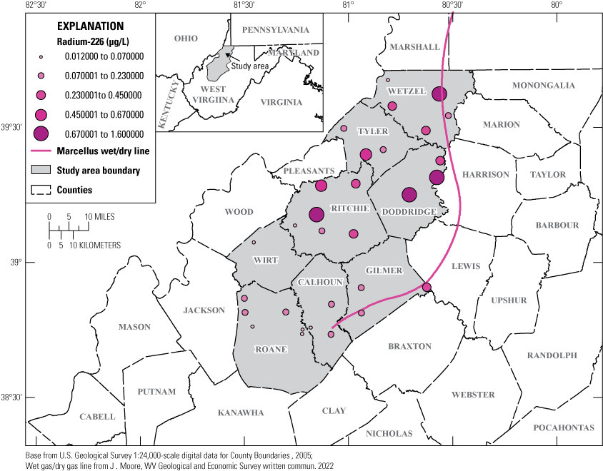
Map showing distribution of radium-226 concentrations for the 30 wells sampled in the wet gas dominated part of the Marcellus Shale oil and gas play in northwestern West Virginia.
Groundwater Age Tracers (CFCs, SF6, and Tritium results)
Groundwater age tracers (CFCs, SF6) were analyzed at 17 of the 30 wells sampled (Haase and others, 2022). The dissolved concentrations of the tracers were corrected for recharge temperature, excess air, and nitrification based on the nitrogen argon (N2/Ar) ratios using the Unsaturated Air (UA) model (Heaton and Vogel, 1981). Concentrations of all the age tracer results were greater than the analytical detection limits for all wells sampled indicating that water recharged after 1950 comprised a substantial fraction of each sample, as CFCs were not used substantially until the late 1940s. This was corroborated by tritium activities greater than 1 TU for all samples, indicating that the samples were predominately young (post 1950s) water (Lindsey and others, 2019). The most reliable age tracer is SF6 because all the samples in this study had very low oxygen or were anoxic, and levels of nitrate, iron, and the presence of methane indicated reducing conditions that potentially degraded all of the CFC tracers to varying degrees. CFC-11 was degraded in most samples to levels that could not be used for dating. There were a few samples with tracer partial pressures greater than those of the atmosphere, or with apparent CFC-113 age younger than the CFC-12 apparent age, (CFC-113: Wet-0114, Wet-0140, and Dod-0070; SF6: Dod-0070, and Rit-0128). The CFC-12 and CFC-113 piston flow ages are roughly correlated with each other and SF6, though they are biased 20 to 30 years older than the SF6, indicating that the CFC tracers in the study experienced similar decay rates. Several sites showed much larger differences in SF6 concentrations (Tyl-0095, Dod-0068, and Tyl-0100), which could indicate locally higher CFC degradation rates or contributions from a non-atmospheric SF6 source. Given that this is observed in other sites in the dataset, the apparent age of these sites is assigned from the CFC-12 age, subtracting the 27-year offset due to degradation. Overall, the combined observation of CFC degradation and non-atmospheric SF6 makes fitting the age distributions to a specific mixing model impractical and only piston flow ages were used to determine relative differences in residence time.
Geochemistry
Rock water interactions, redox state, bedrock mineralogy, freshwater and saline water mixing interactions, cation exchange, and gas composition of groundwater are all factors affecting the geochemistry of groundwater within the study area. These factors were assessed for this study by graphical and statistical analysis. The following sections of this report describe the geochemical processes occurring within the aquifer.
Methane Geochemistry
There are several relationships in the geochemistry that are potentially relevant to the assessment of measured concentrations of methane in the groundwater in this study. The ratio of calcium to sodium in groundwater generally decreases as water equilibrates with aquifer materials and the concentration of TDS increases (fig. 17). Many of the samples in this study have high calcium to sodium (Ca/Na) ratios and low TDS concentrations, indicating the samples are dominated by recently recharged water, and that deep, long-transit-time sources of groundwater are minor.
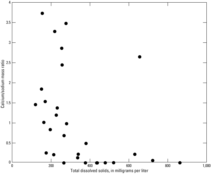
Plot of calcium/sodium mass ratio versus total dissolved solids concentration in the 30 water wells sampled in the wet gas dominated part of the Marcellus Shale oil and gas play in northwestern West Virginia.
Fifteen of the 30 samples had chloride concentrations less than 10 mg/L, limiting the ability to distinguish anion signatures that could characterize samples with halite dissolution, septic runoff, and deep Appalachian basin brine components. A subset of samples had chloride to bromide ratio (Cl/Br) mass ratios between 70 and 200 (fig. 18), indicating deep Appalachian brines mixed with the groundwater (Kessler and others, 1996; Llewellyn and others, 2015; Harkness and others, 2017). The green shaded area between 70 mg/L and 200 mg/L on figure 18 represents the ratios where Appalachian brines are expected to fall (Mullaney and others, 2009). These samples contrast with other common chloride to bromide (Cl/Br) ratios that are typical of halite dissolution (1,000–10,000 from natural and anthropogenic salt sources) and animal waste or sewage (300–1,000), which are the other probable major chloride and bromide sources to groundwater in the area (Mullaney and others, 2009).
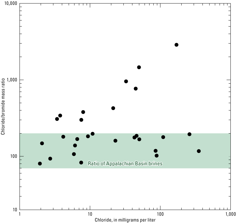
Plot of chloride/bromide mass ratio versus chloride concentration in the 30 wells sampled in the wet gas dominated part of the Marcellus Shale oil and gas play in northwestern West Virginia. The green shaded area indicates the ratio representative of Appalachian basin brines.
Methane and Dissolved Hydrocarbon Composition and Origin
The abundance and sources of dissolved volatile hydrocarbons have long been a topic of study in West Virginia as the state’s abundant coal beds contribute to the presence of hydrocarbons in the state’s groundwater (Mathes and White, 2006; White and Mathes, 2006; Kozar and others, 2012; Chambers and others, 2015; Harkness and others, 2017; McAdoo and Kozar, 2017; Kozar and others, 2020). Natural gas development from the shale resources in the state have renewed interest in the origins of these compounds. Dissolved hydrocarbon concentration data in groundwater can provide information useful in determining the source and geochemical processes responsible for the presence of natural gas in shallow groundwater aquifers. Dissolved methane commonly occurs in groundwater and can originate from microbial activity in the aquifer system or from transport of thermogenic hydrocarbons. The presence of methane in West Virginia’s groundwater is well documented and generally associated with methane from coal beds (Mathes and White, 2006; White and Mathes, 2006; Kozar and others, 2012; Chambers and others, 2015; Harkness and others, 2017; McAdoo and Kozar, 2017; Kozar and others, 2020). As methane is a major component of natural gas recovered from thermally mature shales like the Marcellus Shale in West Virginia and the Utica Shale in Ohio, there is utility in assessing methane concentrations in groundwater before and during well development to establish the baseline conditions, extant sources of methane, and to help understand the relations that changes in water quality might have to surface activity associated with drilling and extraction. (Molofsky and others, 2016; Barth-Naftilan and others, 2018; Woda and others, 2018).
The presence of methane in groundwater could be an indication of contamination and other water-quality issues (Levêque and Burns, 2019; Turley and Caretta, 2020). Functionally, the presence of methane in groundwater has several effects: methane gas can accumulate in enclosed spaces where groundwater is discharged leading to a combustion hazard, it can create unpleasant qualitative characteristics (ebullition and reduced clarity), and it can potentially co-occur with other contaminants that can negatively impact the safety and utility of the water (Borch and Others, 2010). A histogram of the dissolved methane concentrations observed in this study is shown in figure 19 below. Methane concentrations in this study were generally very low, with the most probable concentration being between 0.01 and 0.1 mg/L. No samples exceeded 28 mg/L, but one sample, Rit-0119, exceeded 10 mg/L.
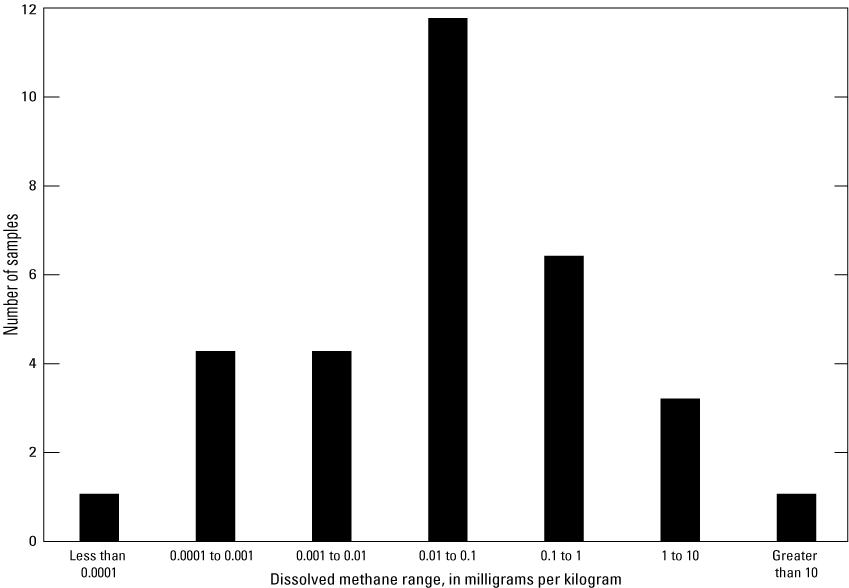
A histogram of the dissolved methane concentrations for the 30 wells sampled in the wet gas dominated part of the Marcellus Shale oil and gas play in northwestern West Virginia.
Methane and other dissolved hydrocarbons originate in groundwater from an array of possible biogenic pathways or from thermogenic sources. Biogenic gas can be generated in situ by multiple reductive pathways and both biogenic and thermogenic gas can be transported from their point of origin by groundwater flow or by resource extraction operations. During transport, compositions of dissolved gas can be modified by mixing with water of different geochemistry and exposure to different redox regimes, resulting in dissolved hydrocarbon compositions having unique signatures (Schoell, 1988; Colosimo and others, 2016). A defining characteristic of biogenic methane is that it does not usually co-occur with concentrations of higher chain hydrocarbons (Cn greater than 1), and therefore has C1/Cn source ratios greater than 1,000. In contrast, thermogenic gas typically has lower C1/Cn ratios, in the range of 10–1,000, with lower ratios representing low thermal maturity wet gas. This is because wet gas has a greater abundance of longer-chained hydrocarbons and higher ratios representing late-stage thermal maturity with lower abundances of higher hydrocarbons (Cn), but, as gas undergoes thermal maturation, the longer-chained hydrocarbons are decomposed to methane, which increases the C1/Cn ratio, compared to that of higher thermal maturity dry gas (Schoell, 1983; Whiticar, 1999; Taylor and others, 2000). After generation, gases can be modified by oxidative processes, fractionation during transport, secondary methanogenesis, biodegradation, and methanotrophy. The cumulative processes result in signatures that can be used to infer the sources, type, and degree of modifications that have acted on a dissolved gas (Whiticar, 1999; Révész and others, 2012; Molofsky and others, 2013; Kozar and others, 2020).
For most of the samples in this study, the C1 to C6 hydrocarbons have characteristics that reflect a biogenic gas signature that has, to varying degrees, undergone methanotrophic oxidation processes during transport. To illustrate these processes, the concentrations of dissolved methane are plotted against the C1/C2 ratio and with the ratios of isobutane to n-butane (fig. 20) and isopentane to n-pentane (fig. 21). This graphic presentation allows the source, mixing, and redox characteristics to be assessed, as trends and groups in isomer fractionation (from approximate source ratios near unity (Lu and others, 2019)) from microbial action and transport are depicted in the same context as dryness and abundance (Molofsky and others, 2013; Kozar and others, 2020).
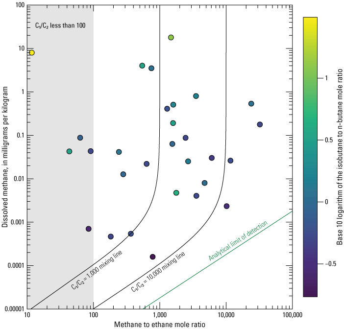
Plot of dissolved methane concentration and the methane to ethane ratio, with a color scale of the ratio of isobutane over n-butane in samples collected from the wet gas dominated part of the Marcellus Shale oil and gas play in northwestern West Virginia.
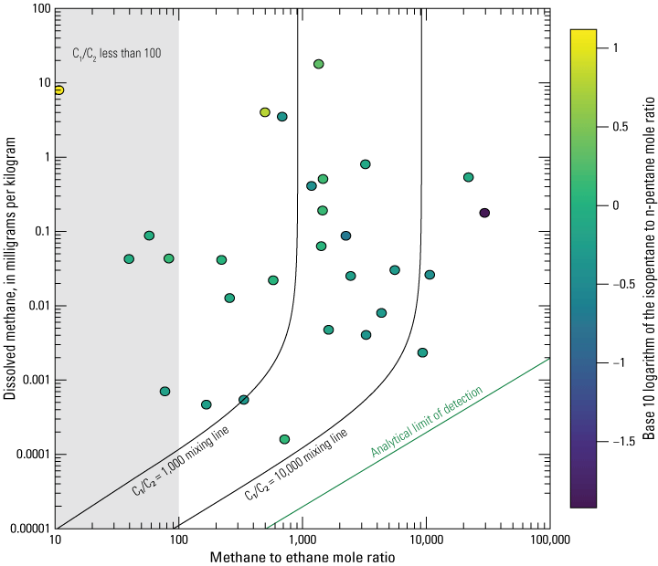
Plot of dissolved methane concentration and methane to ethane ratio, with a color scale of isopentane over n-pentane in the 30 wells sampled in the wet gas dominated part of the Marcellus Shale oil and gas play in northwestern West Virginia.
None of the samples show a characteristic thermogenic cracking pattern among the hydrocarbon ratios, with each successive pair of hydrocarbons (C1/C2, C2/C3, and so on) occurring in ratios in the percent range. Even samples with C1/C2 in the range of a thermogenic source did not have ratios of other (greater than C2) hydrocarbons that indicated a thermogenic origin. Those samples with C1/C2 ratios in the range of 100 were generally of low concentration (less than 0.1 mg/kg), except for sample Cal-0134, which had a concentration of 8.0 mg/kg and had a C1/C2 ratio of 10 but was not accompanied by levels of higher hydrocarbons indicating a proximal thermogenic source of low thermal maturity. The ratios of greater than C2 gases were also less than the range 0.1 ratio expected for thermogenic-sourced gas and were enriched with respect to branched isomers (high isoalkane to n-alkane ratios). This indicates that the gases in this sample had undergone considerable oxidative processing (Prinzhofer and others, 2000; Igari and others, 2007). Figure 20 shows there is no gradient for samples with a high methane and low methane/ethane ratio. The black lines represent the addition of biogenic methane with C1/C2 of 1,000 and 10,000 to background thermogenic gas with C1/C2 between 50 and 100. The green line represents the limit of detection of the measurements.
The plot in figure 21 shows no gradient in pentane isomer ratios for samples with high methane and low ethane/methane ratio. The black lines represent the addition of biogenic methane with C1/C2 of 1,000 and 10,000 to background thermogenic gas with C1/C2 between 50 and 100. The green line represents the limit of detection of the measurements.
The Cl/Br mass ratios of all the samples greater than 1 mg/kg methane are in the range of 70 to 200 (fig. 22), which resemble the anion signatures of Appalachian basin brines (Llewellyn and others, 2015), and coincide with the highest concentrations of methane observed in the study (shaded area on fig. 22). Additionally, all the samples with methane greater than 1 mg/kg were situated in valleys. This follows similar findings in previous studies that showed shallow aquifers in valley bottoms received brines that coincided with the presence of high concentrations of hydrocarbon gases, either from biogenic generation from long flow paths or from introduction into the aquifer by natural Appalachian basin brine movement (Heisig and Scott, 2013; Llewellyn and others, 2015; Colosimo and others, 2016; Molofsky and others, 2016; Harkness and others, 2017; Yan and others, 2017; Woda and others, 2018; Wen and others, 2019). Of the samples with methane concentrations greater than 1 mg/kg, the available groundwater age tracer data indicate that the apparent age was more than 40 years. Further, the low Ca/Na ratios (fig. 23) indicate that long flow paths can coincide with methane occurrence.
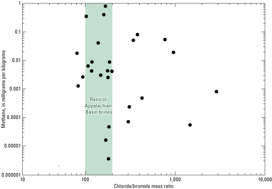
Plot of methane concentration versus chloride/bromide mass ratio in samples collected from the 30 wells sampled in the wet gas part of the Marcellus Shale oil and gas play in northwestern West Virginia.
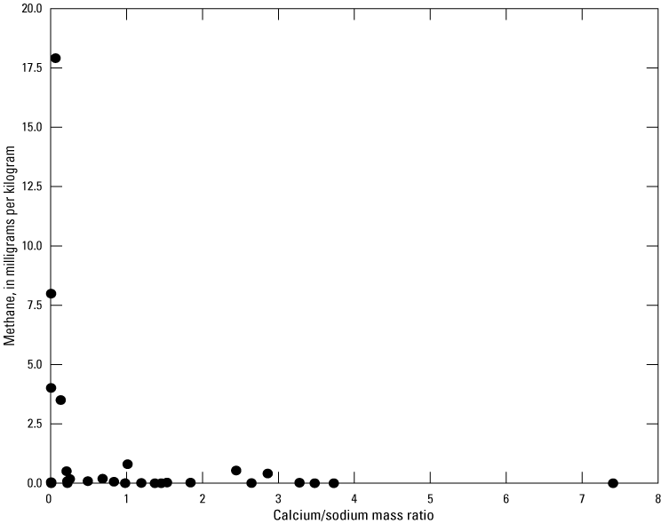
Plot of methane concentration versus calcium to sodium mass ratio in the 30 wells sampled in the wet gas dominated part of the Marcellus Shale oil and gas play in northwestern West Virginia.
In contrast to methane and dissolved hydrocarbons collected in West Virginia’s southern coal field region (Kozar and others, 2020) where fractionation of the branched isomers increased with gas concentration at low C1/C2 ratios, there is not a clear trend in isomeric fractionation (isobutane to n-butane and isopentane to n-pentane) with either methane concentration or methane/ethane ratio, where the ratios of both compounds’ isomers are typically near 1. Though there is considerable variation in the butanes, samples with methane greater than 1 mg/kg tended to display enrichment in branched isomers, whereas samples with lower methane concentrations tended toward enrichment in straight-chain isomers, possibly indicating oxidation or formation pathways for some of the samples with concentrations greater than 1 mg/kg (fig. 24). No patterns were apparent for the pentane or hexane isomers.
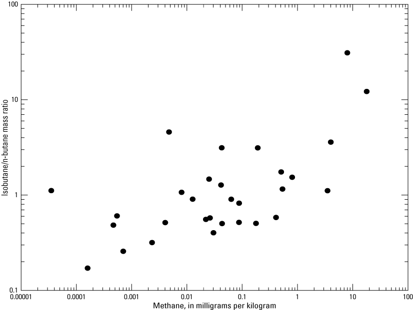
Plot of isobutane to n-butane ratio versus methane concentration in the 30 wells sampled in the wet gas dominated part of the Marcellus Shale oil and gas play in northwestern West Virginia.
Geochemical Evolution of Groundwater
Information on the geochemical processes controlling groundwater evolution in an aquifer system is gathered when data from numerous wells are analyzed together. Boxplots of selected major ions (fig. 25) show clear dominance of the bicarbonate anion and a mixture of calcium, magnesium, and sodium cations, which suggests multiple water-rock interactions in the shallow subsurface are altering solute concentrations from what would be expected in precipitation. Trilinear diagrams (figs. 7, 8B, 8C) also suggest two dominant water types, calcium plus magnesium bicarbonate and sodium plus potassium bicarbonate, with only a few samples showing higher proportions of sulfate for the dominant anion.
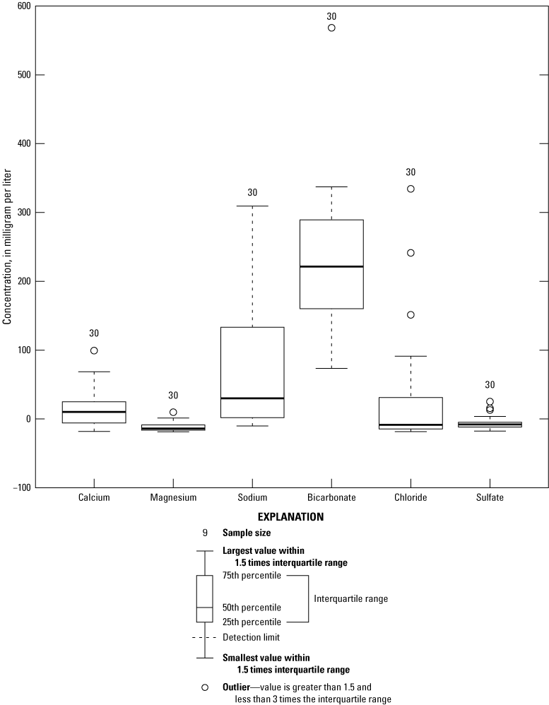
Boxplots of the calcium, magnesium, sodium, bicarbonate, chloride, and sulfate chemistry used to assess the geochemical evolution of groundwater for the 30 wells sampled in the wet gas dominated part of the Marcellus Shale oil and gas play in northwestern West Virginia.
The conceptual model of geochemical evolution for groundwater in this area of West Virginia (fig. 26) starts with recharge from precipitation, is heavily influenced by water-rock interactions, and is classified by three possible redox categories. Precipitation in West Virginia has low dissolved solids, acidic pH, and is capable of dissolving carbonate minerals to buffer acidity during overland flow and infiltration. Precipitation percolates through the soil zone and recharges the saturated zone of the aquifer. Along this path, the chemically aggressive and oxygen-rich water dissolves carbonate minerals and oxidizes sulfides, which releases ions into the solution and increases TDS concentration in the water. Microbes likely mediate oxygen, nitrate, manganese, iron, and sulfate concentrations by preferential electron acceptor utilization through oxic and anoxic redox states (Ouyang and others, 2017).
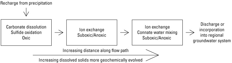
Conceptual model of groundwater geochemical evolution within the wet gas dominated part of the Marcellus Shale oil and gas play in northwestern West Virginia.
The conceptual model of geochemical evolution in the shallow aquifer systems was evaluated by multivariate statistical analysis of the available chemical data for the 30 wells sampled using PCA, comparing significant Spearman’s correlation coefficients (app. 1), graphical analysis, and by computation of SIs for mineral species. The results of the PCA analysis (table 14) show four major hydrogeologic variables – carbonate dissolution, ion exchange, redox, and mixing – controlling the system with 76 percent of the total variance in the dataset explained by these first four principal components. These major hydrogeologic variables are discussed in separate sections that follow. Twenty-six of the most commonly detected variables are represented in the PCA by loadings, which are correlations of individual variables to specific principal components. Positive loadings indicate that as the value of one constituent increases, the value of the correlated constituent also increases, whereas negative loadings indicate that as the value of one constituent increases, the value of the correlated constituent decreases. Spearman’s rho correlation coefficients were found to be significant in this study for values greater than 0.463 and less than -0.463 at a confidence level of 99 percent (p less than 0.01) or between 0.362 and -0.362 at a confidence level of 95 percent (p less than 0.05; table 14; app. 1). Significant Spearman’s rho correlation coefficients for variables not assessed in the principal components model are shown in table 15.
Table 14.
Distribution of eigenvector loadings and significant Spearman’s correlation coefficients for the principal component analysis model.[Communality is a measure of the proportion of the variables variance as a result of the principal components. PC, principal component; p, p-value of statistical significance at a 95-percent confidence level (p less than 0.05) or at a 99-percent confidence level (p less than 0.01); TDS, total dissolved solids; SC, specific conductance; N, nitrogen; Rn-222, radon 222; DO, dissolved oxygen; %, percent, —, percentage not applicable]
Table 15.
Significant Spearman’s correlation coefficients for variables not included in the principal component analysis model.[PC, principal component; p, p-value of statistical significance at a 99 percent confidence level (p less than 0.01); Ra-226, radium 226; --, Spearman’s correlation coefficient not significant (p < 0.01); P, phosphorous; E. coli, Escherichia coli; U234, uranium 234, U238, uranium 238; N, nitrogen; m, meters]
Water-Rock Interactions Controlling Major Ion Concentrations
Dissolution and precipitation of mineral phases present in bedrock and soil zones near a sample site are important in controlling major ion concentrations in groundwater. Various sulfide, sulfate, carbonate, and aluminosilicate minerals common to the bedrock of West Virginia were used to calculate SIs even though the presence of these minerals may vary spatially with depositional environment. If a mineral is present in a sample, the SI indicates the potential of that mineral to precipitate or dissolve. Saturation Indices were computed using the USGS geochemical modeling software, PHREEQC (Parkhurst and Appelo, 2013), and plotted against pH (fig. 27) to identify mineral phases that may affect the solute concentration if the mineral is present.
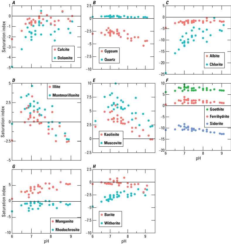
Saturation indices of calcite to dolomite, gypsum to quartz, albite to chlorite, illite or montmorillonite, kaolinite to muscovite, goethite and ferrihydrite to siderite, manganite to rhodochrosite, and barite to witherite phases calculated from the water-quality data for the 30 wells sampled in the wet gas dominated part of the Marcellus Shale oil and gas play in northwestern West Virginia.
Carbonate Dissolution
The first component—carbonate dissolution (table 14)—has significant (p less than 0.01) positive loadings indicative of the geochemical process that increases hardness through carbonate dissolution. These processes include the highest positive loadings for hardness, calcium, and magnesium. Carbonate mineral phases that commonly control these constituents in solution are mostly undersaturated (fig. 27A) throughout the entire pH range in the study area indicating that calcite and dolomite are likely the source of hardness in the shallow aquifer. pH has significant negative loading on the first component which suggests that carbonate dissolution occurs at lower pH water which may have higher dissolved carbon dioxide from recent recharge. The mass of magnesium averages 35 percent of the mass of calcium throughout the study area and figure 28 clearly shows that the mass of calcium is greater than the mass of magnesium at all sites. This is a good indication that calcite dissolution is more important than dolomite dissolution in the addition of hardness and alkalinity to the shallow aquifer system.
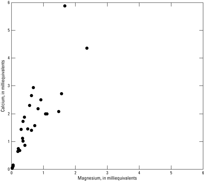
Comparison of the equivalent mass of calcium and magnesium calculated from the water-quality data for the 30 wells sampled in the wet gas dominated part of the Marcellus Shale oil and gas play in northwestern West Virginia.
Occurrence of Trace Elements
The first principal component—carbonate dissolution—also has significant (p less than 0.01) loadings for strontium and barium, which are alkali earth minerals and commonly replace calcium and magnesium in the crystal lattice of carbonate minerals. Like calcium and magnesium, they are subsequently released when these minerals are dissolved (Skougstad and Albert, 1963). It is also possible, to a lesser degree, that barium and strontium concentrations are increased due to the dissolution of strontianite or witherite (fig. 27H), but these minerals are less common.
Positive loadings on principal component one for iron and manganese at a lower level of significance (p less than 0.05) may be due to oxidation of sulfide minerals, but the dissolved oxygen is generally low, and this may not be the case in many of these samples. Siderite and rhodochrosite (iron and manganese carbonate minerals) are undersaturated in these samples which means they may dissolve and possibly be a source (figs. 27F, G), but more information on the study area mineralogy is needed to confirm if they are present in the aquifer. Uranium mobilization is more common in shallow oxic parts of aquifers and increases with uranyl-carbonate complexation (Langmuir, 1978). Positive loading of uranium on principal component one at a lower level of significance (p less than 0.05) provides evidence that oxygen may be more prevalent than indicated by the absence of dissolved oxygen loading in the PCA, and oxidation of sulfides may increase iron and manganese in less evolved groundwater where carbonate dissolution is the dominant process. Figure 27H shows that barite is at saturation throughout the study area. With the dissolution of sulfide minerals, it would be expected that sulfate would be higher than is observed but with high loadings of barium on component one, it is possible that sulfate is removed from the solution through precipitation of barite, or in reducing conditions where reduction to hydrogen sulfide could occur.
Ion Exchange
The second component—ion exchange (table 14)—has significant (p less than 0.01) positive loadings for TDS, specific conductance, alkalinity, sodium, chloride, bromide, and positive loading at the 95 percent confidence level for pH. In systems where calcite dissolution is a major hydrochemical process, calcium and magnesium should increase with increasing bicarbonate at the pH range observed throughout the study area, but figure 29 shows that several samples have calcium and magnesium concentrations that are lower than would be expected with increasing bicarbonate.
Alkalinity is used to calculate bicarbonate, increases in solutions from dissolution of carbonate minerals, and is expected to load on the first principal component with calcium and magnesium but, instead, significantly loads on the second component and has no significant correlation with calcium or manganese (p less than 0.01, app. 1). Alkalinity and pH are both positively correlated with sodium (p less than 0.01, app. 1) and normally have a dependent relationship but are not significantly correlated with each other (p less than 0.01, app. 1) in this dataset. Calcium and magnesium are negatively correlated with sodium (p less than 0.01, app. 1) which means sodium generally increases in concentration as calcium and magnesium decrease. These observations indicate that there is either a source of alkalinity that is unaccounted for or calcium and magnesium are being replaced in more evolved water, likely through ion exchange with sodium.
Comparing the calcium, magnesium, and sodium to bicarbonate ratios (fig. 29) shows that sodium is 10 to 100 times higher in the study area than would be expected from halite dissolution alone. The ratio of calcium plus magnesium to bicarbonate is mostly less than one and close to zero in some samples, which indicates that if bicarbonate comes primarily from carbonate dissolution, then calcium and magnesium are being removed from the system, likely by ion exchange with sodium.
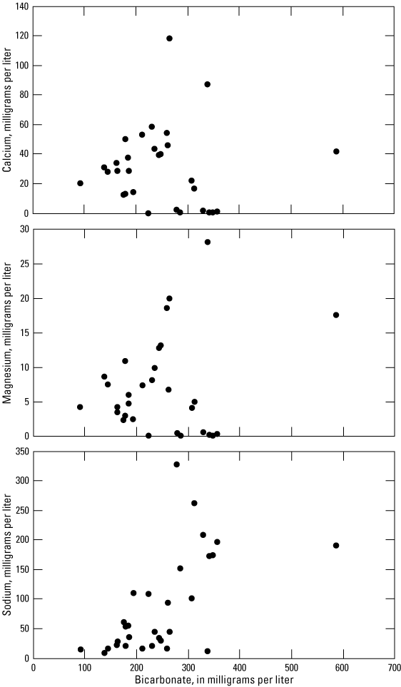
Plot showing calcium, magnesium, and sodium increasing with bicarbonate concentrations for the 30 wells sampled in the wet gas dominated part of the Marcellus Shale oil and gas play in northwestern West Virginia.
Observations of analyte ratios and correlations between certain constituents coupled with the loadings on the second component (table 14) suggest that ion exchange is an important geochemical process controlling calcium, magnesium, and sodium concentrations in the system. Specifically, as the groundwater moves along the flow path and dissolves more carbonate minerals, calcium, magnesium, and bicarbonate increase in solution. As pH and alkalinity increase, calcium and magnesium begin to exchange with sodium on clay minerals. Removing calcium and magnesium from the solution promotes more carbonate dissolution and the formation of sodium bicarbonate-type waters. Continued carbonate dissolution as a result of ion exchange is also a likely explanation for why values of alkalinity and pH generally increase with increasing sodium concentrations (fig. 30).
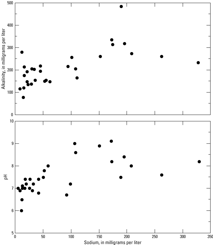
Plot showing alkalinity and pH increasing with sodium concentration for the 30 wells sampled in the wet gas dominated part of the Marcellus Shale oil and gas play in northwestern West Virginia.
Assuming increased TDS is an indication of more evolved groundwater, as described by figure 26, carbonate dissolution likely occurs throughout the entire flow path and ion exchange is initiated when the flow path intersects clay mineral exchange points. Figure 31 shows specific conductance, pH, sodium, bicarbonate, calcium, and magnesium concentrations plotted against increasing TDS. As described by the conceptual geochemical model, TDS is expected to increase with greater geochemical evolution of groundwater along a flow path. Specific conductance and sodium have a positive monotonic relationship (p less than 0.01) with TDS and continually increase throughout groundwater flow paths. Bicarbonate and pH initially increase with TDS until TDS reaches approximately 400 mg/L, which may indicate the point where dissolution of carbonate minerals is reduced or the system becomes saturated with respect to calcite and subsequently precipitates carbonate minerals. Except for a few samples, sodium continues to increase after TDS reaches approximately 300 mg/L, while calcium and magnesium concentrations generally stop increasing at this point, indicating the influence of ion exchange in more evolved water.
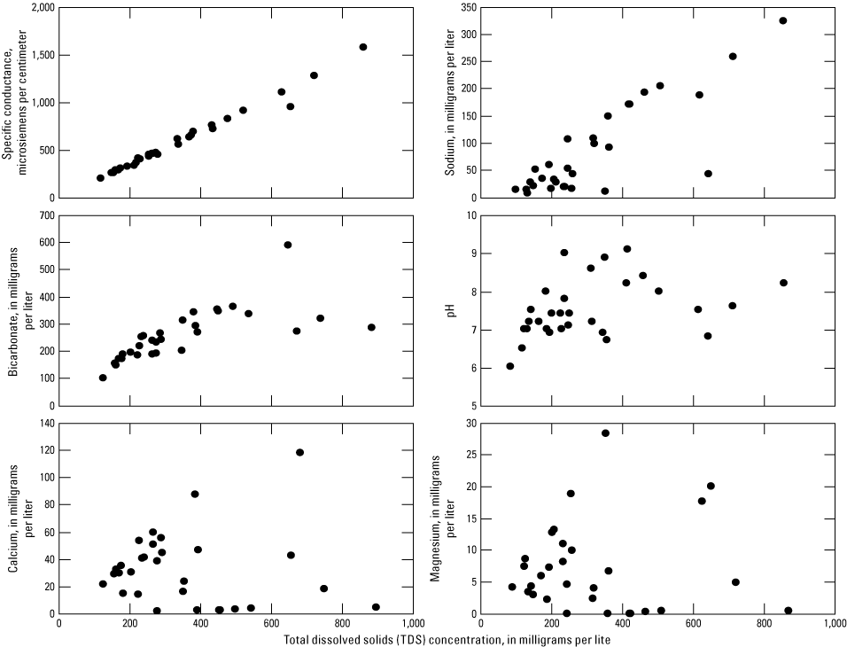
Figure showing selected field parameters and major ions plotted against total dissolved solids (TDS) concentration for the 30 wells sampled in the wet gas dominated part of the Marcellus Shale oil and gas play in northwestern West Virginia.
Reduction and Oxidation Processes
The third principal component (table 14) is representative of ions that are controlled by redox processes and has significant (p less than 0.01) positive loadings for ammonia, iron, manganese, radon, and arsenic. The lack of significant negative loading for dissolved oxygen indicates that redox processes are likely catalyzed by microorganisms and ion concentrations are controlled by preferential electron acceptor utilization. The ecological succession of terminal electron-accepting processes is the preferential order of the most energetically favorable and naturally available electron acceptor for microbial metabolism. The order of reduction processes starts with oxygen, followed by nitrate in anoxic conditions, followed by manganese, ferric iron, sulfate, and carbon dioxide. The most common electron donor in groundwater systems is dissolved organic carbon. This process is further explained by McMahon and Chapelle (2008).
Following methods outlined by McMahon and Chapelle (2008) for categorizing and identifying redox processes according to threshold concentrations of major electron acceptors (table 16), each site was classified by a redox category and possible redox processes that may be controlling ion concentrations. An important observation (table 17) is that many of these sites are classified as mixed and several meet the criteria for multiple redox processes. This is possibly due to open well bore construction in the fractured-rock aquifers and mixing of several redox zones in long open intervals which may reduce the usefulness of using threshold concentrations to identify specific redox processes (McMahon and Chapelle, 2008; McMahon and others, 2019).
Table 16.
Threshold concentrations for identifying redox processes.[Redox process based on water quality criteria defined by McMahon and Chapelle (2008). mg/L, milligram per Liter; O2, oxygen; ≥, greater than or equal to; --, no process identified; <, less than; redox, reduction oxidation; NO3− - N, nitrate as nitrogen; Mn2+, manganese; Fe2+, ferrous iron; SO42-, sulfate]
Table 17.
Dominant redox processes determined from threshold concentrations of major electron acceptors.[Redox process based on water quality criteria defined by McMahon and Chapelle (2008). mg/L, milligram per Liter; redox, reduction oxidation; Wet, Wetzel County; O2, oxygen; Wir, Wirt County; NO3−, nitrate; Fe (III), ferric iron; SO42−, sulfate; Rit, Ritchie County; Tyl, Tyler County; Mn (IV), same as Mn4+; Dod, Doddridge County; Gil, Gilmer County; Roa, Roane County; Cal, Calhoun County; --, no process identified]
Nevertheless, the data (table 17) clearly show that Mn (IV) and Fe (III) reduction is an important process at several sites. In the aquifer, Mn (IV) is likely in the mineral form of a manganese oxide and Fe (III) is likely in the mineral form of a ferric oxyhydroxide. Upon microbial reduction of Mn (IV) and Fe (III) mineral species, manganese and iron are released into solution as anions (Mn2+ and Fe2+). Soluble arsenate complexes can adsorb on the surfaces of Mn (IV) and Fe (III) oxyhydroxides and subsequently release arsenic to solution upon microbial reduction and dissolution of these minerals.
McMahon and others (2019) have shown that manganese concentrations are significantly higher in wells with shallow (less than 5 m) depth-to-open-interval and depth-to-water due to increased transport of dissolved organic carbon from the soil zone and subsequent microbial reduction of manganese oxides. From the PCA model, well depth has a negative loading (p less than 0.01) on the third principal component which suggests that shallower wells have higher concentrations of iron and manganese that may originate from oxidation of sulfide minerals but could be controlled by microbial mediated reduction of Mn (IV) and Fe (III) oxides or oxyhydroxides. The negative loading (p less than 0.01) of uranium further supports the evidence that the third principal component is representative of sites with low oxygen because uranium mobilization is more common in the shallow oxic parts of the aquifer and increases with uranyl-carbonate complexation (Langmuir, 1978). Redox control on ion concentrations is clearly complex in the shallow aquifer system of the study area and may need additional study and analysis to fully understand.
Influence from Appalachian Basin Brines
The fourth principal component—mixing (table 14)—has significant (p less than 0.01) positive loadings for methane, ethane, and bromide which may be indicative of deeper Appalachian basin brines influencing the shallow aquifer system. Negative loadings for dissolved oxygen and sulfate suggest reducing conditions where sulfate reduction may be important. The previous section on Methane Geochemistry showed that a subset of sites had bromide/chloride ratios that meet the criteria for brine classification, but the chloride concentrations are relatively low and the proportion of brine in these samples is likely small. With these data, it is difficult to determine the source of the brine signature and whether it is from natural upwellings, legacy wells, or recent oil and gas activity. There is a significant (p less than 0.01, app. 1) correlation between the fourth principal component and the total number of wells within 500 m which suggests that either these wells are impacted by oil and gas activity, or oil and gas activity is more pronounced around these groundwater wells because target drilling formations are closer to the surface and the wells are impacted by natural brines closer to the shallow system.
Summary
Thirty primarily rural residential wells were sampled for a broad range of chemical constituents to provide a baseline dataset of groundwater-quality data for current assessment and future comparison and to assess the effect, or lack thereof, of oil and gas development on shallow groundwater quality within the study area. A primary impetus for this project was concern that trace metals, radionuclides, or other contaminants present in water from unregulated residential water wells may pose a health threat to individuals that rely on these sources for their water supply. For that reason, groundwater-quality data collected for this study are compared to public drinking-water standards, even though those regulations are not enforceable for rural residential water supplies. A majority of the constituents analyzed in this study did not exceed any of the aforementioned standards. There were several notable exceptions, most of which were not unexpected based on previous studies.
Turbidity exceeded the 5 Nephelometric Turbidity Unit (NTU) U.S. Environmental Protection Agency (EPA) maximum contaminant level (MCL) drinking water standard in 2 of 30 (7 percent) wells sampled and exceeded the 1 NTU surface water treatment rule (SWTR) treatment technique (TT) standard in 12 of 30 (40 percent) wells sampled. Turbidity is common in many wells in West Virginia and may be related to iron oxyhydroxide precipitates, sediment carried into the aquifers from the shallow soil zone due to improperly constructed or cased wells or transported to the aquifer in shallow stress relief fracture zones. The minimum, maximum, mean, and median turbidity levels for the 30 wells sampled were 0.30, 60.0, 3.21, and 0.85. NTUs, respectively.
For the wells sampled, 5 (17 percent) had pH that were outside the 6.5–8.5 EPA secondary maximum contaminant level (SMCL) for pH, and of those 5 sites, 4 (80 percent) were indicative of alkaline water and only 1 (20 percent) was indicative of acidic water. The minimum, maximum, mean, and median pH levels for the 30 wells sampled were 6.0, 9.1, 7.5, and 7.4 standard pH units, respectively.
The Langelier Saturation Index (LSI) is a measure of calcite saturation and can be used as an indicator of the potential for calcium scale to form in plumbing. Of the 30 wells sampled, 27 sites (90 percent) had an LSI less than -0.5, indicative of corrosive waters, 3 sites (10 percent) had LSI values in the indeterminate range, and none (0 percent) of the wells sampled had an LSI value of an alkaline scale-forming water.
The corrosivity of water alone is insufficient to assess whether water from a particular well has the potential to promote galvanic corrosion (PPGC). Therefore, PPGC was computed for the 30 wells sampled. Of the 30 wells sampled, none (0 percent) had a PPGC that classified as high, 26 (87 percent) were classified as moderate, and 4 (13 percent) were classified as low. Since the PPGC classification is based partly on total alkalinity, the moderate to high levels of alkalinity present in groundwater in the study area buffer the water and reduce the potential to promote galvanic corrosion in public and residential water systems in the study area.
Both total coliform bacteria and Escherichia coli (E. coli) were detected in groundwater samples from the 30 wells sampled. Total coliforms, which are a broad class of indicator bacteria, are common in groundwater in West Virginia and were detected in 26 of the 30 wells (87 percent) sampled. The presence of total coliform bacteria in groundwater are a potential indicator of surface contamination, but E. coli bacteria are indicative of fecal contamination of groundwater from either human or animal sources. Eleven of the 30 (37 percent) wells sampled had detections of E. coli bacteria, and the presence of E. coli in groundwater may be considered an indicator of other related pathogens such as viruses. In these cases, chlorination, ozonation, or ultraviolet (UV) light treatment may be appropriate to kill potential pathogenic microorganisms.
Total dissolved solids (TDS), which are a measure of the amount of dissolved constituents in a water sample and are commonly related to water hardness, exceeded the 500-milligram per liter (mg/L) EPA secondary maximum contaminant level (SMCL) in 5 of 30 (17 percent) wells sampled. Overall 40 percent of the sites sampled had hardness representative of hard to very hard water, but most of the wells sampled had water that was considered moderately hard to soft. Soft water can make it difficult for soap to work effectively and water that is too hard can contribute to scale deposits in water heaters and plumbing lines.
Sodium, chloride, fluoride, and sulfate are very common constituents in groundwater within the study area. Sulfate and chloride in water can impart a salty taste to water at concentrations greater than 250 mg/L. Sulfate and chloride concentrations in the study area were generally low, none (0 percent) of the wells sampled contained sulfate in concentrations exceeding the EPA SMCL of 250 mg/L and only 2 of 30 (7 percent) wells sampled contained chloride in excess of the EPA SMCL. Sodium has an EPA health-based value (HBV) of 20 mg/L for individuals who are on a sodium-restricted diet for blood pressure or other health reasons. Sodium concentrations were elevated in a large proportion of the wells sampled, with 24 of 30 (80 percent) exceeding the 20-mg/L HBV. Fluoride in high concentrations can cause mottling or discoloration of teeth. The EPA SMCL for fluoride is 2.0 mg/L and only 1 of 30 (3 percent) wells sampled contained fluoride (2.86 mg/L) greater than this amount.
Manganese, aluminum, and iron were prevalent contaminants detected in the groundwater samples collected for this study with many of the samples exceeding the proposed SMCL drinking-water standards for these constituents: 14 of 30 (47 percent) sites for manganese, 7 of 30 (23 percent) sites for aluminum, and 5 of 30 (16.7 percent) wells sampled for iron exceeding the proposed 50-, 2.0-, and 300-micrograms per liter (µg/L) SMCL drinking-water standards, respectively. Two of the 30 wells sampled (7 percent) had concentrations of manganese that exceeded the 300-µg/L U.S. Geological Survey (USGS) health-based screening level (HBSL) and none of the wells sampled exceeded the 1,600-µg/L EPA drinking water equivalent level (DWEL), which is based on a lifetime exposure level. There are no applicable HBSLs or DWELs for iron or aluminum in drinking water. The median, maximum, and minimum concentrations of iron for the 30 wells sampled were 31.1 µg/L, 5,150 µg/L, and less than the 10-µg/L method detection limit, respectively. The median, maximum, and minimum concentrations of manganese for the 30 wells sampled were 35.2 µg/L, 527 µg/L, and less than the 0.4-µg/L method detection limit, respectively. The maximum concentration of aluminum for the 30 wells sampled was 101 µg/L, but the median and minimum aluminum concentrations for wells sampled was less than the 3.0 µg/L method detection limit, respectively.
Lead also can be a problem constituent with respect to human health in some aquifers, but none (0 percent) of the wells sampled for this study exceeded the EPA TT drinking water standard. The EPA MCL goal (MCLG) for lead is 0, and 23 of 30 (77 percent) of wells sampled contained lead at detectable concentrations. However, the maximum lead concentration detected was only 0.998 µg/L with median and minimum concentrations of 0.077 µg/L and less than the 0.020 µg/L method detection limit, respectively.
Arsenic is a potential contaminant of concern with respect to human health within the study area, with 7 of 30 (23 percent) of the wells sampled exceeding the 10-µg/L EPA MCL health-based drinking water standard. The EPA MCLG for arsenic is 0 µg/L, and 29 of 30 wells sampled contained detectable concentrations of arsenic. The maximum, median, and minimum arsenic concentrations for the wells sampled were 31.4 µg/L, 2.40 µg/L and less than the 0.19-µg/L method detection limit, respectively.
Mercury was only detected at 1 of 30 (3 percent) wells sampled, exceeding the EPA MCLG of 0 µg/L for mercury but did not exceed either the EPA MCL or DWEL. The concentration of mercury for the one site sampled with a detectable concentration was only 0.008 µg/L. None of the 30 wells sampled had barium, beryllium, antimony, cadmium, chromium, copper, selenium, silver, or zinc concentrations exceeding the EPA MCLs, MCLGs, SMCLs, DWELs, or molybdenum and nickel concentrations exceeding EPA DWELs or USGS HBSLs. Median concentrations of barium and zinc were 222 and 4.70 µg/L, and median concentrations of antimony, beryllium, cadmium, chromium, copper, selenium, and silver were all low, with median concentrations for the 30 wells sampled of less than the method detection levels of 0.06, 0.01, 0.03, 0.5, 0.4, 0.05, 1.0, µg/L, respectively. Except for barium, median concentrations were typically at or below the method detection limits.
Methane and other dissolved hydrocarbons are potentially explosive combustible gases that are commonly related with the production and development of oil and gas, which is a dominant land-use in the study area, so the potential for these gases to be present in groundwater in the study area was assessed. There are no EPA drinking-water standards for methane gas or other dissolved hydrocarbons except for benzene. The EPA MCL and MCLG goal for benzene are 5.0 and 0.0 milligrams per kilogram (mg/kg), respectively. Benzene was detected at 11 of 30 (37 percent) wells sampled, all at very low concentrations. The maximum benzene concentration was only 9.84 × 10⁻⁶ mg/kg and none of the wells sampled (0 percent) had concentrations of benzene in excess of the EPA MCL drinking water standard.
Only 1 of 30 (3 percent) wells sampled for methane gas had a concentration (17.9 mg/kg) exceeding the 10-mg/L U.S. Office of Surface Mining Reclamation and Enforcement (OSMRE) level of concern (LOC), and none exceeded the 28-mg/L immediate action level (IAL). Median, minimum, and maximum concentrations of methane gas for the 30 wells sampled were 0.042, 3.51 × 10⁻⁵, and 17.9 mg/kg, respectively.
Radium-224, radium-226, radium-228, uranium, uranium-234, uranium-235, uranium-238, and gross alpha and gross beta radioactivity were analyzed for the 30 wells sampled. Radon-222 was only analyzed in 28 of the wells sampled (2 radon-222 samples were lost in shipment). These constituents are not uncommon in bedrock in the study area but are more commonly associated with dark shales such as the Marcellus Shale, which is the target formation for horizontal well oil and gas development within the study area. For the wells sampled, all 28 (100 percent; 2 of the 30 were lost in shipment) met or exceeded the EPA-proposed 300-picocuries per liter (pCi/L) MCL for radon, but none exceeded the 4,000-pCi/L alternate maximum contaminant level (AMCL), which is applicable to public drinking water systems that have adopted radon mitigation programs. Sites with radon gas concentrations exceeding the 300-pCi/L proposed MCL have the potential for airborne concentrations of radon to exceed the 4-pCi/L indoor air standard. Inhalation of radon can cause lung cancer and the 4-pCi/L indoor air standard is based on an inhalation standard. Therefore, homeowners whose wells have dissolved radon gas concentrations exceeding 300 pCi/L may be advised to test their indoor air concentrations. The mean radon concentration was 1,461 pCi/L, the median was 1,450 pCi/L, and the maximum and minimum radon concentrations were 2,910 and 320 pCi/L, respectively.
Wilcoxon Signed Rank Tests determined that there were statistically significant differences in concentrations of calcium, magnesium, potassium, silica, and turbidity for Dunkard Group wells compared with the combined data for the Conemaugh Group and Monongahela Formation wells. Results of the Wilcoxon Signed Rank Test of statistical comparison of populations by constituent show that the overall turbidity, calcium, magnesium, and potassium concentrations are higher for wells sampled in the Dunkard Group than for wells sampled in the combined Conemaugh Group and Monongahela Formation. Concentrations of sodium are highest in groundwater sampled from the Conemaugh Group and Monongahela Formation.
The depth of wells also can affect groundwater quality, as deeper wells typically contain lower dissolved oxygen levels than shallower wells or wells with short casings. Dissolved oxygen, or the lack thereof, is a primary factor controlling reduction-oxidation (redox) processes in groundwater. For wells sampled for this study, shallower wells less than 95 feet (ft) deep had slightly higher dissolved oxygen, iron, manganese, radon-222, and ammonia concentrations than wells greater than or deeper than 95 ft, which had slightly higher concentrations of calcium, magnesium, bicarbonate, and uranium. Median concentrations of dissolved oxygen, iron, manganese, radon-222, and ammonia for shallow wells were 0.6 mg/L, 66.6 µg/L, 62.7 µg/L, 1,615 pCi/L, and 0.120 µg/L, respectively, whereas deeper wells had much lower median concentrations of dissolved oxygen, iron, manganese, radon-222, and ammonia of 0.4 mg/L, 12.2 µg/L, 6.3 µg/L, 1,075 pCi/L, and 0.070 µg/L, respectively. Median concentrations of calcium, magnesium, bicarbonate, and uranium for shallow wells were 20.4 mg/L, 3.55 mg/L, 185 mg/L, and less than 0.033 mg/L, respectively, whereas deeper wells had slightly higher median concentrations of calcium, magnesium, bicarbonate, and uranium of 39.9 mg/L, 7.43 mg/L, 262 mg/L, and less than 0.166 mg/L, respectively.
There were statistically significant differences in valley and upland wells for total coliform bacteria, calcium, magnesium, ammonia, nitrate, radon-222, uranium, copper, manganese, molybdenum, selenium, ethane, and methane. Concentrations of dissolved oxygen, calcium, magnesium, nitrate, uranium, and copper were greater in upland wells compared to valley wells, and constituents of ammonia, radon-222, iron, manganese, and molybdenum were greater in valley wells as compared to upland wells. As was evident for chemical constituent concentrations for deep and shallow wells, the primary process likely responsible for the differences in groundwater quality between upland and valley wells are redox processes.
Groundwater-quality data for the wells sampled also were assessed with respect to the proximity to nearby oil and gas wells. Processes associated with the drilling of oil and gas wells, production of oil and gas, and associated maintenance and upgrade of wells within the study area have been postulated to possibly affect groundwater quality within the study area. There was a statistically significant difference based on Wilcoxon Signed Rank Test in radium-226, barium, and ethane concentrations with respect to the density of oil and gas wells present within a 500-meter (m) radius around the rural residential wells sampled for the study. Residential wells sampled that had four or fewer oil and gas wells surrounding the residential wells sampled had statistically lower concentrations of radium-226, bromide, and ethane than for residential wells sampled that had 5 or more oil and gas wells in a 500-m radius of the wells sampled. Since methane is the dominant gas produced in the region, whether the elevated concentrations of radium-226, bromide, and ethane are related to oil and gas development or whether the elevated concentrations are related to natural geochemical processes is uncertain. A larger more robust dataset using similar methods would help to assess whether the differences are due to oil and gas development or due to natural geochemical processes.
Groundwater age tracers (chlorofluorocarbons, sulfur hexafluoride) were sampled at 17 of the 30 sites. All the tracers were greater than the detection limit for all wells sampled indicating that water recharged after the 1950s comprised a substantial fraction of each sample. This was corroborated by tritium activities greater than 1 tritium unit for all samples, indicating that the samples were predominately young, post 1950s in age.
Except for methane, the dissolved hydrocarbon concentrations were very low, and the maximum benzene concentration was only 9.84 × 10⁻⁶ mg/kg, which is equivalent to a non-detect using analytical methods for which the MCL standard was designed. There are several relationships in the geochemistry that are relevant to the measured concentrations of methane in the groundwater in this study. First, the ratio of calcium to sodium in groundwater decreases as water equilibrates with aquifer materials and the concentration of TDS increases. Many of the samples in this study have high calcium to sodium (Ca/Na) ratios and low TDS concentrations, indicating they are dominated by recently recharged water, and that deep, long transit time sources are minor. A subset of samples had chloride to bromide mass ratios between 70 and 200, indicating deep Appalachian basin brines mixed with the shallow groundwater. For most of the samples in this study, the C1 to C6 hydrocarbons have characteristics that reflect a biogenic gas signature that has, to varying degrees, undergone oxidation processes during transport. Six of the samples have low C1/C2 ratios that are indicative of a thermogenic origin, though these samples do not show a characteristic thermogenic cracking pattern among the higher (C2+) hydrocarbons, indicating that the gas composition has undergone biological processing during natural migration that has obscured its source characteristics.
The Cl/Br mass ratios of all the samples greater than 1 mg/kg methane are in the range of 100–200, which resemble the anion signatures of Appalachian basin brines. Additionally, all methane wells with methane concentrations greater than 1 mg/kg were situated in valleys. This follows similar findings of prior studies that show that shallow aquifers in valley bottoms can receive brines that may coincide with the presence of high concentrations of hydrocarbon gases, either from biogenic generation from long flow paths or from being carried into the aquifer by natural Appalachian basin brine movement.
The conceptual model of geochemical evolution for groundwater in this area of West Virginia starts with precipitation, is heavily influenced by water-rock interactions, and was classified by three possible redox categories. Precipitation in West Virginia has low dissolved solids, acidic pH, and is capable of dissolving carbonate minerals to buffer acidity. Precipitation percolates through the soil zone and becomes recharge in the saturated zone of the aquifer. Along this path, the chemically aggressive and oxygen-rich water dissolves carbonate minerals and oxidizes sulfides which releases ions into the solution and increases dissolved solids concentration in the water. Microbes likely mediate oxygen, nitrate, manganese, iron, and sulfate concentrations by preferential electron acceptor utilization through oxic and anoxic redox states.
The conceptual model of geochemical evolution in the shallow aquifer systems was evaluated by multivariate statistical analysis of the available chemical data for the 30 wells sampled using multivariate principal components analysis (PCA), comparing significant Spearman’s correlation coefficients, graphical analysis, and by computation of saturation indices (SIs) for mineral species.
The first component is indicative of the geochemical process that increases hardness through carbonate dissolution. Carbonate mineral phases that commonly control these constituents in solution are mostly undersaturated throughout the entire pH range in the study area, indicating that calcite and dolomite are likely the source of hardness in the shallow aquifer. The first principal component also has statistically significant (p less than 0.01) loadings for strontium and barium which are alkali earth minerals and commonly replace calcium and magnesium in the crystal lattice of carbonate minerals. Like calcium and magnesium, they are subsequently released when these minerals are dissolved (Skougstad and Albert, 1963).
The second component indicates that there is either a source of alkalinity that is unaccounted for or calcium and magnesium are being replaced in more evolved water. Comparing the sodium chloride ratio with the calcium plus magnesium and bicarbonate ratio shows that sodium is 20 to 100 times higher in the study area than would be expected from halite dissolution alone, further supporting the premise for cation exchange. The ratio of calcium plus magnesium to bicarbonate is mostly less than one and close to zero in some samples which indicates that if bicarbonate comes primarily from carbonate dissolution, then calcium and magnesium are being removed from the system. Specifically, as the groundwater moves along the flow path and dissolves more carbonate minerals, calcium, magnesium, and bicarbonate increase in solution. The pH increases with increasing alkalinity and calcium and magnesium begin to exchange with sodium on clay minerals. Continued carbonate dissolution as a result of ion exchange is also a likely explanation for why values of alkalinity and pH generally increase with increasing sodium concentrations.
The third principal component is representative of ions that are controlled by redox processes and has statistically significant (p less than 0.01) positive loadings for ammonia, iron, manganese, and arsenic. The lack of significant negative loading for dissolved oxygen indicates that redox processes are likely catalyzed by microorganisms and ion concentrations are controlled by preferential electron acceptor utilization. Mn (IV) and Fe (III) reduction is an important process at several sites. In the aquifer, Mn (IV) is likely in the form of a manganese oxide and Fe (III) is likely in the form of a ferric oxyhydroxide. Upon microbial reduction of Mn (IV) and Fe (III) species, manganese and iron are released into solution as anions (Mn2+ and Fe2+).
The fourth principal component has significant (p less than 0.01) positive loadings for methane, ethane, and bromide and a significant (p less than 0.05) positive loading for chloride which is indicative of the shallow aquifer system mixing with deeper Appalachian basin brine. There is a statistically significant (p less than 0.01) correlation between the fourth principal component and the total number of oil and gas wells within 500-m, which suggests that either these wells are impacted by oil and gas activity or oil and gas activity is greater around these wells because target drilling formations are closer to the surface and the wells are impacted by natural brines closer to the shallow system.
References Cited
American Public Health Association, American Water Works Association, and Water Environment Foundation, 2018, Standard methods for the examination of water and wastewater: Enzyme substrate coliform test, accessed February 5, 2018, at https://www.standardmethods.org/action/doSearch?AllField=Enzyme+Substrate+Coliform+Test.
Back, W., 1966, Hydrochemical facies and ground water flow patterns in northern part of Atlantic Coastal Plain: U.S. Geological Survey Professional Paper 498–A, p. A1–A42, accessed February 7, 2019, at https://pubs.er.usgs.gov/publication/pp498A.
Bader, J.S., Mathes, M.V., and Shultz, R.A., 1997, Ground-water hydrology of the area bordering the Ohio River between Chester and Waverly, West Virginia: U.S. Geological Survey Open-File Report 95–710, 61 p., accessed February 5, 2018 at, https://doi.org/10.3133/ofr95710.
Barth-Naftilan, E., Sohng, J., and Saiers, J.E., 2018, Methane in groundwater before, during, and after hydraulic fracturing of the Marcellus Shale: Proceedings of the National Academy of Sciences of the United States of America, v. 115, no. 27, p. 6970–6975, accessed February 7, 2019, https://doi.org/10.1073/pnas.1720898115.
Belitz, K., Jurgens, B.C., and Johnson, T.D., 2016, Potential corrosivity of untreated groundwater in the United States: U.S. Geological Survey Scientific Investigations Report 2016–5092, 16 p., accessed February 7, 2019, at https://doi.org/10.3133/sir20165092.
Berg, T.M., Edmunds, W.E., Geyer, A.R., Glover, A.D., Hoskins, D.M., MacLachlan, D.B., Root, S.I., Sevon, W.D., Socolow, A.A., Miles, C.E., and Kuchinski, J.G., 1980, Geologic map of Pennsylvania: Pennsylvania Department of Environmental Resources, Bureau of Topographic and Geologic Survey State Geologic Map, scale 1:250,000, 2 sheets.
Blake, B.M., Jr., Cross, A.T., Eble, C.F., Gillespie, W.H., and Pfefferkorn, H.W., 2002, Selected plant megafossils from the Carboniferous of the Appalachian region, United States, in Hills, L.V., Henderson, C.M., and Bamber, E.W., eds., Carboniferous and Permian of the World—Canadian Society of Petroleum Geologists Memoir, v. 19, p. 259–335, stratigraphic column accessed April 3, 2020, at https://www.wvgs.wvnet.edu/www/coal/coal_images/WVGES_CoalStratChartPennsylvanianBeds.pdf.
Borch, T., Kretzschmar, R., Kappler, A., Van Cappellen, P., Ginder-Vogel, M., Voegelin, A., and Campbell, K., 2010, Biogeochemical redox processes and their impact on contaminant dynamics: Environmental Science and Technology, v. 44, no. 1, p, 15–23, accessed September 23, 2022, at https://doi.org/10.1021/es9026248.
Busenberg, E., and Plummer, L.N., 1992, Use of chlorofluorocarbons as hydrologic tracers and age-dating tools—The alluvium and terrace system of central Oklahoma: Water Resources Research, v. 28, no. 9, p. 2257–2283, accessed February 7, 2019, https://doi.org/10.1029/92WR01263.
Busenberg, E., and Plummer, L.N., 2000, Dating young groundwater with sulfur hexaflluoride—Natural and anthropogenic sources of sulfur hexafluoride: Water Resources Research, v. 36, no. 10, p. 3011–3030, accessed February 7, 2019. https://doi.org/10.1029/2000WR900151.
Callaghan, T., Fleeger, G.M., Barnes, S., and Dalberto, A., 1998, Groundwater flow on the Appalachian Plateau of Pennsylvania, in Brady, K.B.C., Smith, M.W., and Schueck, J., eds., Coal mine drainage prediction and pollution prevention in Pennsylvania: Harrisburg, Pa., Pennsylvania Department of Environmental Protection, 5600-BK-DEP2256 8/98, chap. 2, p. 2-1 to 2-39, accessed February 12, 2018, at https://files.dep.state.pa.us/mining/BureauOfMiningPrograms/BMPPortalFiles/Coal_Mine_Drainage_Prediction_and_Pollution_Prevention_in_Pennsylvania.pdf.
Cecil, C.B., Stanton, R.W., Neuzil, S.G., DuLong, F.T., Ruppert, L.F., and Pierce, B.S., 1985, Paleoclimate controls on late Paleozoic sedimentation and peat formation in the central Appalachian Basin (USA): International Journal of Coal Geology, v. 5, no. 1–2, p. 195–230, accessed February 7, 2019. https://doi.org/10.1016/0166-5162(85)90014-X.
Chambers, D.B., Kozar, M.D., Messinger, T., Mulder, M.L., Pelak, A.J., and White, J.S., 2015, Water quality of groundwater and stream base flow in the Marcellus Shale gas field of the Monongahela River Basin, West Virginia, 2011–12 (ver. 1.1, June 25, 2015): U.S. Geological Survey Scientific Investigations Report 2014–5233, 76 p., accessed February 7, 2019, at https://doi.org/10.3133/sir20145233.
Chambers, D.B., Kozar, M.D., White, J.S., and Paybins, K.S., 2012, Groundwater quality in West Virginia, 1993–2008: U.S. Geological Survey Scientific Investigation Report 2012–5186, 47 p., accessed February 7, 2019, at https://pubs.usgs.gov/sir/2012/5186/.
Colosimo, F., Thomas, R., Lloyd, J.R., Taylor, K.G., Boothman, C., Smith, A.D., Lord, R., and Kalin, R.M., 2016, Biogenic methane in shale gas and coal bed methane—A review of current knowledge and gaps: International Journal of Coal Geology, v. 165, p. 106–120, accessed February 7, 2019. https://doi.org/10.1016/j.coal.2016.08.011.
Cozzarelli, I.M., Skalak, K.J., Kent, D.B., Engle, M.A., Benthem, A., Mumford, A.C., Haase, K., Farag, A., Harper, D., Nagel, S.C., Iwanowicz, L.R., Orem, W.H., Akob, D.M., Jaeschke, J.B., Galloway, J., Kohler, M., Stoliker, D.L., and Jolly, G.D., 2017, Environmental signatures and effects of an oil and gas wastewater spill in the Williston Basin, North Dakota: Science of the Total Environment, v. 579, p. 1781–1793, accessed November 17, 2020. https://doi.org/10.1016/j.scitotenv.2016.11.157.
Eggleston, J.R., 2004, History of West Virginia Mineral Industries—Oil and Gas: West Virginia Geological and Economic Survey web page, accessed April 7, 2021, at www.wvgs.wvnet.edu/www/geology/geoldvog.htm.
Eltschlager, K.K., Hawkins, J.W., Ehler, W.C., and Baldassare, F., 2001, Technical measures for the investigation and mitigation of fugitive methane hazards in areas of coal mining: Pittsburgh, Pa., Office of Surface Mining Reclamation and Enforcement, 124 p., accessed July 7, 2022, at https://ntrl.ntis.gov/NTRL/dashboard/searchResults/titleDetail/PB2002106133.xhtml.
Esri, 2020, ArcGIS for Desktop Release 10.8.1: Redlands, Calif., Esri, accessed January 30, 2020, at https://support.esri.com/en/Products/Desktop/arcgis-desktop/arcmap/10-8-1.
Fedorko, N., and Skema, V., 2013, A review of the stratigraphy and stratigraphic nomenclature of the Dunkard Group in West Virginia and Pennsylvania, USA: International Journal of Coal Geology, v. 119, p. 2–20, accessed February 7, 2019. https://doi.org/10.1016/j.coal.2013.07.016.
Friel, E.A., Ehlke, T.A., Hobba, W.A., Ward, S.M., Jr., and Schultz, R.A., 1987, Hydrology of area 8, eastern coal province, West Virginia and Ohio: U.S. Geological Survey Open-file. Report 84-463, 78 p., accessed February 7, 2019, at https://doi.org/10.3133/ofr84463.
Haase, K.B., Kozar, M.D., McAdoo, M.A., and Ried, L.T., 2022, Dataset of C1-C6 dissolved trace hydrocarbon measurements in the western “Wet Gas” part of the Marcellus Shale Oil and Gas Play in West Virginia, U.S.A. collected between June and August 2018: U.S. Geological Survey data release, accessed September 30, 2022, at https://doi.org/10.5066/P9L98L0Y.
Haase, K.B., Busenberg, E., Plummer, L.N., Casile, G., and Sanford, W.E., 2014, Measurements of HFC-134a and HCFC-22 in groundwater and unsaturated-zone air—Implications for HFCs and HCFCs as dating tracers: Chemical Geology, v. 385, p. 117–128, accessed February 7, 2019. https://doi.org/10.1016/j.chemgeo.2014.07.016.
Hanshaw, B.B., and Back, W., 1979, Major geochemical processes in the evolution of carbonate—Aquifer systems: Journal of Hydrology, v. 43, no. 1–4, p. 287–312, accessed February 7, 2019. https://doi.org/10.1016/0022-1694(79)90177-X.
Harkness, J.S., Darrah, T.H., Warner, N.R., Whyte, C.J., Moore, M.T., Millot, R., Kloppmann, W., Jackson, R.B., and Vengosh, A., 2017, The geochemistry of naturally occurring methane and saline groundwater in an area of unconventional shale gas development: Geochimica et Cosmochimica Acta, v. 208, p. 302–334, accessed November 17, 2020. https://doi.org/10.1016/j.gca.2017.03.039.
Harlow, G.E., Jr., and LeCain, G.D., 1993, Hydraulic characteristics of, and ground-water flow in, coal-bearing rocks of southwestern Virginia: U.S. Geological Survey Water Supply Paper 2388, 36 p., accessed February 8, 2019, at https://pubs.usgs.gov/wsp/wsp_2388/.
Heaton, T.H.E., and Vogel, J.C., 1981, “Excess air” in groundwater: Journal of Hydrology, v. 50, p. 201–216, accessed April 4, 2014. https://doi.org/10.1016/0022-1694(81)90070-6.
Heisig, P.M., and Scott, T.-M., 2013, Occurrence of methane in groundwater of south-central New York State, 2012—Systematic evaluation of a glaciated region by hydrogeologic setting: U.S. Geological Survey Scientific Investigations Report 2013–5190, 32 p., accessed February 8, 2019, at https://doi.org/10.3133/sir20135190.
Hem, J.D., 1992, Study and interpretation of the chemical characteristics of natural water: U.S. Geological Survey Water Supply Paper 2254, 264 p., accessed February 8, 2019, at https://pubs.usgs.gov/wsp/wsp2254/.
Hendryx, M., and Ahern, M.M., 2009, Mortality in Appalachian coal mining regions—The value of statistical life lost: National Library of Medicine Public Health Reports, v. 124, no. 4, p. 541–550, accessed February 8, 2019, at https://www.ncbi.nlm.nih.gov/pmc/articles/PMC2693168/.
Homer, C., Dewitz, J., Yang, L., Jin, S., Danielson, P., Xian, G., Coulston, J., Herold, N., Wickham, J., and Megown, K., 2015, Completion of the 2011 national land cover database for the conterminous United States—Representing a decade of land cover change information: Bethesda, Md., American Society for Photogrammetric Engineering and Remote Sensing, v. 81, no. 5, p. 345–354, accessed January 27, 2020, at https://catalog.data.gov/dataset/nlcd-2011-database.
IDEXX, 2019, Overview and resources for the Colilert method for processing and quantification of total coliform and E. coli bacteria: IDEXX web page, accessed May 15, 2018, at https://www.idexx.com/en/water/water-products-services/colilert/.
Igari, S.-I., Maekawa, T., and Suzuki, Y., 2007, Pentane and hexane isomers in natural gases from oil and gas fields in Akita, Niigata and Hokkaido, Japan—Determination factor in their isomer ratios: Geochemical Journal, v. 41, no. 1, p. 57–63, accessed February 8, 2019, https://doi.org/10.2343/geochemj.41.57.
Kessler, S.E., Martini, A.M., Appold, M.S., Walter, L.M., Huston, T.J., and Furman, F.C., 1996, Na-Cl-Br systematics of fluid inclusions from Mississippi Valley-type deposits, Appalachian Basin—Constraints on solute origin and migration paths: Geochimica et Cosmochimica Acta, v. 60, no. 2, p. 225–233, accessed November 17, 2020, https://doi.org/10.1016/0016-7037(95)00390-8.
Kozar, M.D., McAdoo, M.A., and Haase, K.B., 2020, Groundwater quality and geochemistry of West Virginia’s southern coal fields (ver. 1.1, March 2020): U.S. Geological Survey Scientific Investigations Report 2019−5059, 78 p., accessed April 1, 2021 at https://doi.org/10.3133/sir20195059.
Kozar, M.D., and Mathes, M.V., 2001, Aquifer-characteristics data for West Virginia: U.S. Geological Survey Water-Resources Investigations Report 01–4036, 74 p., accessed February 11, 2019, at https://pubs.usgs.gov/wri/wri01-4036/.
Kozar, M.D., McCoy, K.J., Britton, J.Q., and Blake, B.M.B., Jr., 2012, Hydrogeology, groundwater flow, and groundwater quality of an abandoned underground coal-mine aquifer, Elkhorn area, West Virginia: West Virginia Geological and Economic Survey Bulletin B-46, 103 p., accessed February 11, 2019, at http://downloads.wvgs.wvnet.edu/pubcat/docs/Bulletin_46_Hydrogeology,%20Groundwater%20Abandoned%20Coal%20Mine%20Aquifer,%20Elkhorn,%20WV_(2012).pdf.
Langmuir, D., 1978, Uranium solution-mineral equilibria at low temperatures with applications to sedimentary ore deposits: Geochemica et Cosmochimica Acta, v. 42, no. 6, part A, p. 547–569, accessed February 11, 2019, at https://doi.org/10.1016/0016-7037(78)90001-7.
Levêque, J.G., and Burns, R.C., 2019, Water quality perceptions and natural resources, Extraction - A matter of geography?: Journal of Environmental Management, v. 234, p. 379–386, accessed November 17, 2020. https://doi.org/10.1016/j.jenvman.2018.11.126.
Lindsey, B.D., Jurgens, B.C., and Belitz, K., 2019, Tritium as an indicator of modern, mixed, and premodern groundwater age: U.S. Geological Survey Scientific Investigations Report 2019–5090, 18 p., accessed November 11, 2020 at https://doi.org/10.3133/sir20195090.
Llewellyn, G.T., Dorman, F., Westland, J.L., Yoxtheimer, D., Grieve, P., Sowers, T., Humston-Fulmer, E., and Brantley, S.L., 2015, Evaluating a groundwater supply contamination incident attributed to Marcellus Shale gas development: Proceedings of the National Academy of Sciences of the United States of America, v. 112, no. 20, p. 6325–6330, accessed November 11, 2020. https://doi.org/10.1073/pnas.1420279112.
Lorenz, D.L., 2018, USGS-R/smwrQW – Tools for censored data analysis, Version 0.7.14, accessed February 7, 2019, at https://rdrr.io/github/USGS-R/smwrQW/.
Lorenz, D.L., and Diekoff, A.L., 2017, smwrGraphs—An R package for graphing hydrologic data, version 1.1.2: U.S. Geological Survey Open-File Report 2016–1188, 17 p., accessed February 11, 2019, at https://doi.org/10.3133/ofr20161188.
Lu, S., Li, J., Xue, H., Chen, F., Xu, Q., Wang, M., Wenbaio, L., and Pang, X., 2019, Pyrolytic gaseous hydrocarbon generation and the kinetics of carbon isotope fractionation in representative model compounds with different chemical structures: Geochemistry, Geophysics, Geosystems, v. 20, p. 1773–1793, accessed November 11, 2020. https://doi.org/10.1029/2018GC007722.
Mathes, M.V., and White, J.S., 2006, Methane in West Virginia ground water: U.S. Geological Survey Fact Sheet 2006–3011, 2 p., accessed February 11, 2019, at https://pubs.usgs.gov/fs/2006/3011/.
McAdoo, M.A., and Kozar, M.D., 2017, Groundwater-quality data associated with abandoned underground coal mine aquifers in West Virginia, 1973–2016—Compilation of existing data from multiple sources: U.S. Geological Survey Data Series 1069, 7 p., accessed February 7, 2019 at https://doi.org/10.3133/ds1069.
McAuley, S.D., and Kozar, M.D., 2006, Ground-water quality in unmined areas and near reclaimed surface coal mines in the northern and central Appalachian coal regions, Pennsylvania and West Virginia: U.S. Geological Survey Scientific Investigations Report 2006–5059, 57 p., accessed February 11, 2019, at https://pubs.usgs.gov/sir/2006/5059/.
McMahon, P.B., Belitz, K., Reddy, J.E., and Johnson, T.D., 2019, Elevated manganese concentrations in United States groundwater, role of land surface-soil-aquifer connections: Environmental Science & Technology, v. 53, no. 1, p. 29–38, accessed February 9, 2019, https://doi.org/10.1021/acs.est.8b04055.
McMahon, P.B., and Chapelle, F.H., 2008, Redox processes and water quality of selected principal aquifer systems: Ground Water, v. 46, no. 2, p. 259–271, accessed February 7, 2019. https://doi.org/10.1111/j.1745-6584.2007.00385.x.
Milici, R.C., 2004, Assessment of Appalachian Basin oil and gas resources—Carboniferous coal-bed gas total petroleum system: U.S. Geological Survey Open-file Report 2004–1272, 98 p., accessed February 7, 2019 at https://doi.org/10.3133/ofr20041272.
Molofsky, L.J., Connor, J.A., McHugh, T.E., Richardson, S.D., Woroszylo, C., and Alvarez, P.J., 2016, Environmental factors associated with natural methane occurrence in the Appalachian Basin: Groundwater, v. 54, no. 5, p. 656–668, February 11, 2019, at https://doi.org/10.1111/gwat.12401.
Molofsky, L.J., Connor, J.A., Wylie, A.S., Wagner, T., and Farhat, S.K., 2013, Evaluation of methane sources in groundwater in northeastern Pennsylvania: Ground Water, v. 51, no. 3, p. 333–349, accessed February 11, 2019, https://doi.org/10.1111/gwat.12056.
Mullaney, J.R., Lorenz, D.L., and Arntson, A.D., 2009, Chloride in groundwater and surface water in areas underlain by the glacial aquifer system, northern United States: U.S. Geological Survey Scientific Investigations Report 2009–5086, accessed February 19, 2019. https://doi.org/10.3133/sir20095086.
Myers, D.N., and Sylvester, M.A., 2014, Fecal indicator bacteria in National field manual for the collection of water-quality data: U.S. Geological Survey Techniques of Water-Resources Investigations, book 9, chap. 7.1 (09-A7.1), 73 p., accessed February 12, 2018, at https://pubs.er.usgs.gov/publication/twri09A7.1.
National Oceanic and Atmospheric Administration, 2022, Climatological station normals for 1991–2020 for Middlebourne, West Virginia, accessed July 12, 2022, at https://www.ncei.noaa.gov/access/us-climate-normals/#dataset=normals-monthly&timeframe=30&location=WV&station=USC00465963.
Nguyen, C.K., Clark, B.N., Stone, K.R., and Edwards, M.A., 2011, Role of chloride, sulfate, and alkalinity on galvanic lead corrosion: Corrosion, v. 67, no. 6, 9 p., accessed February 11, 2019, at https://doi.org/10.5006/1.3600449.
Norman, J.E., Toccalino, P.L., and Morman, S.A., 2018, Health-based screening levels for evaluating water-quality data (2d ed.): U.S. Geological Survey web page, accessed February 11, 2019, at https://water.usgs.gov/water-resources/hbsl/.
Orem, W.H., Varonka, M.S., Crosby, L.M., Haase, K.B., Loftin, K.A., Hladik, M., Akob, D.M., Tatu, C., Mumford, A.C., Jaeschke, J.B., Bates, A.L., Schell, T., and Cozzarelli, I.M., 2017, Organic geochemistry and toxicology of a stream impacted by unconventional oil and gas wastewater disposal operations: Applied Geochemistry, v. 80, p. 155–167, accessed November 17, 2020, https://doi.org/10.1016/j.apgeochem.2017.02.016.
Otton, J.K., 1992, The geology of radon—General Interest Publications of the U.S. Geological Survey: U.S. Department of the Interior, 30 p., accessed July 12, 2022 at https://pubs.usgs.gov/gip/7000018/report.pdf.
Ouyang, B., Akob, D.M., Dunlap, D., and Renock, D., 2017, Microbially mediated barite dissolution in anoxic brines: Applied Geochemistry, v. 76, p. 51–59, accessed February 11, 2019. https://doi.org/10.1016/j.apgeochem.2016.11.008.
Papp, L., Palcsu, L., Major, Z., Rinyu, L., and Tóth, I., 2012, A mass spectrometric line for tritium analysis of water and noble gas measurements from different water amounts in the range of microlitres and millilitres: Isotopes in Environmental and Health Studies, v. 48, no. 4, p. 494–511, accessed November 17, 2020. https://doi.org/10.1080/10256016.2012.679935.
Parkhurst, D.L., and Appelo, C.A.J., 2013, Description of input and examples for PHREEQC version 3—A computer program for speciation, batch-reaction, one-dimensional transport, and inverse geochemical calculations: U.S. Geological Survey Techniques and Methods 6‒A43, book 6, chap. A43, 497 p., accessed February 11, 2019, at https://pubs.usgs.gov/tm/06/a43/.
Piper, A.M., 1944, A graphic procedure in the geochemical interpretation of water-analyses: Eos (Washington, D.C.), v. 25, no. 6, p. 914–923, accessed February 11, 2019. https://doi.org/10.1029/TR025i006p00914.
Prinzhofer, A., Mello, M.R., and Takaki, T., 2000, Geochemical characterization of natural gas—A physical multivariable approach and its applications in maturity and migration estimates: AAPG Bulletin, v. 84, no. 8, p. 1152–1172, accessed February 11, 2019. https://doi.org/10.1306/A9673C66-1738-11D7-8645000102C1865D.
Puente, C., 1985, West Virginia Ground-Water Resources, in National Water Summary 1984, Hydrologic events, selected water-quality trends, and ground water resources: U.S. Geological Survey Water-Supply Paper 2275, p. 439–446, accessed July 12, 2022, at https://pubs.usgs.gov/wsp/2275/report.pdf.
R Core Team, 2017, R: A language and environment for statistical computing: Vienna, Austria R Foundation for Statistical Computing, accessed February 11, 2019, at https://www.R-project.org/.
Renock, D., Landis, J.D., and Sharma, M., 2016, Reductive weathering of black shale and release of barium during hydraulic fracturing: Applied Geochemistry, v. 65, p. 73–86, accessed February 11, 2019. https://doi.org/10.1016/j.apgeochem.2015.11.001.
Revelle, W., 2022, Package ‘psych’: Procedures for psychological, psychometric, and personality research: Evanston, Ill., Northwestern University, 445 p., accessed July 12, 2022 at https://cran.r-project.org/web/packages/psych/psych.pdf.
Révész, K.M., Breen, K.J., Baldassare, A.J., and Burruss, R.C., 2012, Carbon and hydrogen isotopic evidence for the origin of combustible gases in water-supply wells in north-central Pennsylvania: Applied Geochemistry, v. 27, no. 1, p. 361–375, accessed February 11, 2019. https://doi.org/10.1016/j.apgeochem.2011.12.002.
Rowan, E.L., Engle, M.A., Kirby, C.S., and Kraemer, T.F., 2011, Radium content of oil- and gas-field produced waters in the northern Appalachian Basin (USA)—Summary and discussion of data: U.S. Geological Survey Scientific Investigations Report 2011–5135, 31 p., accessed February 7, 2019 at https://doi.org/10.3133/sir20115135.
Ryder, R.T., Crangle, R.D., Jr., Trippi, M.H., Sweezy, C.S., Lentz, E.E., Rowan, E.L., and Hope, R.S., 2009, Geologic Cross Section D-D’ through the Appalachian Basin from the Findlay Arch, Sandusky County, Ohio, to the Valley and Ridge Province, Hardy County, West Virginia: U.S. Geological Survey Scientific Investigations Map 3067, 52 p., 2 pls.
Schlosser, P., Stute, M., Dörr, H., Sonntag, C., and Münnich, K.O., 1988, Tritium/3He dating of shallow groundwater: Earth and Planetary Science Letters, v. 89, no. 3–4, p. 353–362, accessed November 17, 2020. https://doi.org/10.1016/0012-821X(88)90122-7.
Schoell, M., 1988, Multiple origins of methane in the Earth: Chemical Geology, v. 71, no. 1–3, p. 1–10, accessed February 11, 2019. https://doi.org/10.1016/0009-2541(88)90101-5.
Skougstad, M.W., and Albert, H.C., 1963, Occurrence and distribution of strontium in natural water: U.S. Geological Survey Water Supply Paper 1496–D, 50 p., accessed February 9, 2019, at https://pubs.er.usgs.gov/publication/wsp1496D.
Stoner, J.D., 1983, Probable hydrologic effects of subsurface mining: Ground Water Monitoring and Remediation, v. 3, no. 1, p. 128–137, accessed July 12, 2022. https://doi.org/10.1111/j.1745-6592.1983.tb00874.x.
Taylor, S.W., Sherwood Lollar, B., and Wassenaar, I., 2000, Bacteriogenic ethane in near-surface aquifers—Implications for leaking hydrocarbon well bores: Environmental Science & Technology, v. 34, no. 22, p. 4727–4732, accessed February 9, 2019. https://doi.org/10.1021/es001066x.
Turley, B., and Caretta, M.A., 2020, Household water security – An analysis of water affect in the context of hydraulic fracturing in West Virginia, Appalachia: Water, vol. 12, no. 147, 22 p., accessed April 2, 2021, at https://doi.org/10.3390/w12010147.
U.S. Environmental Protection Agency, 2019, Drinking water contaminants regulations: U.S. Environmental Protection website, accessed February 12, 2019, at https://www.epa.gov/dwreginfo/drinking-water-regulations.
U.S. Environmental Protection Agency, 2022a, National primary drinking water regulations: U.S. Environmental Protection Agency website, accessed, at https://www.epa.gov/ground-water-and-drinking-water/national-primary-drinking-water-regulations.
U.S. Environmental Protection Agency, 2022b, Secondary drinking water standards—Guidance for nuisance chemicals: U.S. Environmental Protection Agency website, accessed, at https://www.epa.gov/ground-water-and-drinking-water/national-primary-drinking-water-regulations.
U.S. Geological Survey, 2006, Collection of water samples (ver. 2.0): U.S. Geological Survey Techniques of Water-Resources Investigations, book 9, chap. A4, September 2006, accessed February 12, 2018, at https://pubs.water.usgs.gov/twri9A4/.
U.S. Geological Survey, 2020, Water use data for West Virginia–2015, in USGS water data for the Nation: U.S. Geological Survey National Water Information System database, accessed March 12, 2020, at http://doi.org/10.5066/F7P55KJN. [Site information directly accessible at https://waterdata.usgs.gov/wv/nwis/water_use/.]
U.S. Geological Survey, 2021, USGS water data for the Nation: U.S. Geological Survey National Water Information System database, accessed March 12, 2021 at http://doi.org/10.5066/F7P55KJN.
U.S. Geological Survey and Association of American State Geologists, 2020a, National geologic map database for the Conemaugh Group, accessed April 3, 2020, at https://ngmdb.usgs.gov/Geolex/UnitRefs/ConemaughRefs_1192.html.
U.S. Geological Survey and Association of American State Geologists, 2020b, National geologic map database for the Monongahela Formation, accessed April 3, 2020, at https://ngmdb.usgs.gov/Geolex/Units/Monongahela_2826.html.
Wen, T., Woda, J., Marcon, V., Niu, X., Li, Z., and Brantley, S.L., 2019, Exploring how to use groundwater chemistry to identify migration of methane near shale gas sells in the Appalachian Basin: Environmental Science & Technology, v. 53, no. 15, p. 9317–9327, accessed November 17, 2020, https://doi.org/10.1021/acs.est.9b02290.
West Virginia Geological and Economic Survey, 2020a, Oil and gas summary statistics query page: West Virginia Geological and Economic Survey database, accessed March 12, 2020, at http://www.wvgs.wvnet.edu/www/datastat/ogsummary/start2.asp.
West Virginia Geological and Economic Survey, 2020b, Updated oil and gas well data: West Virginia Geological and Economic Survey database, accessed March 12, 2020, at http://www.wvgs.wvnet.edu/www/news/ogdvd1.html.
West Virginia Geological and Economic Survey, 2020c, West Virginia mine information database system: West Virginia Geological and Economic Survey, accessed March 18th, 2020 at https://www.wvgs.wvnet.edu/www/mids/main.php.
West Virginia Geological and Economic Survey, 2022, West Virginia stratigraphy: West Virginia Geological and Economic Survey web page, accessed August 1st, 2022, at http://www.wvgs.wvnet.edu/www/geology/stratigraphy/stratigraphy.htm.
West Virginia Office of Miner’s Health Safety and Training, 2020, Annual reports: West Virginia Office of Miner’s Health Safety and Training website, accessed July 12, 2022, at https://minesafety.wv.gov/annual-reports/.
White, J.S., and Mathes, M.V., 2006, Dissolved-gas concentrations in ground water in West Virginia, 1997–2005: U.S. Geological Survey Data Series 156, 8 p., accessed February 12, 2019, at https://pubs.usgs.gov/ds/2005/156/.
Whiticar, M.J., 1999, Carbon and hydrogen isotope systematics of bacterial formation and oxidation of methane: Chemical Geology, v. 161, no. 1–3, p. 291–314, accessed February 12, 2019. https://doi.org/10.1016/S0009-2541(99)00092-3.
Wilde, F.D., Radtke, D.B., Gibs, J., and Iwatsubo, R.T., eds., 2004, Processing of water samples (ver. 2.2, February 2009): U.S. Geological Survey Techniques of Water-Resources Investigations, book 9, chap. A5, accessed February 12, 2018, at https://pubs.water.usgs.gov/twri9A5/.
Woda, J., Wen, T., Oakley, D., Yoxtheimer, D., Engelder, T., Castro, M.C., and Brantley, S.L., 2018, Detecting and explaining why aquifers occasionally become degraded near hydraulically fractured shale gas wells: Proceedings of the National Academy of Sciences of the United States of America, v. 115, no. 49, p. 12349–12358, accessed February 7, 2019. https://doi.org/10.1073/pnas.1809013115.
Yan, B., Stute, M., Panettieri, R.A., Jr., Ross, J., Mailloux, B., Neidell, M.J., Soares, L., Howarth, M., Liu, X., Saberi, P., and Chillrud, S.N., 2017, Association of groundwater constituents with topography and distance to unconventional gas wells in NE Pennsylvania: Science of the Total Environment, v. 577, p. 195–201, accessed February 12, 2019. https://doi.org/10.1016/j.scitotenv.2016.10.160.
Appendix 1. Correlation matrix showing Spearman’s correlation coefficients of statistical significance at a confidence interval of 99 percent for 58 variables, including 45 chemical constituents, 4 principal component analysis scores, 8 land use classifications, and well depth
Conversion Factors
U.S. customary units to International System of Units
International System of Units to U.S. customary units
Temperature in degrees Celsius (°C) may be converted to degrees Fahrenheit (°F) as follows:
°F = (1.8 ×°C) + 32.
Temperature in degrees Fahrenheit (°F) may be converted to degrees Celsius (°C) as follows:
°C = (°F − 32) / 1.8.
Datum
Vertical coordinate information is referenced to the North American Vertical Datum of 1988 (NAVD 88).
Horizontal coordinate information is referenced to the North American Datum of 1983.
Altitude, as used in this report, refers to distance above the vertical datum.
Supplemental Information
Specific conductance is given in microsiemens per centimeter at 25 degrees Celsius (μS/cm at 25 °C).
Concentrations of chemical constituents in water are given in milligrams per liter (mg/L), micrograms per liter (μg/L), or milligrams per kilogram (mg/kg).
Concentrations of dissolved hydrocarbons within this report are given in mg/kg, which for freshwater is equivalent to mg/L.
Activities for radioactive constituents in water are given in picocuries per liter (pCi/L).
Results for measurements of tritium are expressed in tritium units (TUs).
Note to USGS users: Use of hectare (ha) as an alternative name for square hectometer (hm2) is restricted to the measurement of small areas of land or water. Use of liter (L) as a special name for cubic decimeter (dm3) is restricted to the measurement of liquids and gases. No prefix other than “milli” is used with liter.
Abbreviations
3He
helium-3
AED
atomic emission detector
AMCL
alternate maximum contaminant level
Bbl
barrel
bls
below land surface
C1 to C6
hydrocarbons methane, ethane, ethene, ethyne, propane, propene, propyne, n-butane, isobutane, 1-butene, n-pentane, isopentane, 2- and 3-methylpentane, hexane, and benzene
Ca/Na
calcium to sodium ratio
CaCO3
calcium carbonate
CDC
Centers for Disease Control and Prevention
CFC
chlorofluorocarbon
(ft3/s)/mi2
cubic foot per second per square mile
Cl/Br
chloride to bromide ratio
Cn
higher chain hydrocarbons
CSMR
chloride to sulfate mass ratio
DEM
digital elevation model
DWEL
drinking water equivalent level
E. coli
Escherichia coli
EPA
U.S. Environmental Protection Agency
fg/kg
femtogram per kilogram
FID
flame ionization detector
ft
foot
ft/s
foot per second
ft3/s
cubic foot per second
g
gram
gal
gallon
gal/min
gallon per minute
gal/min/ft
gallon per minute per foot
GC-FID/AED
gas chromatrography-flame ionization detector and atomic emission detector
HBSL
health-based screening level
HBV
health-based value
IAL
immediate action level
IAP
ion activity product
ICP
inductively coupled plasma
in/yr
inch per year
K
Kelvin
Ksp
thermodynamic solubility product
LOC
level of concern
LSI
Langelier saturation index
m
meter
MCF
thousand cubic foot
MCL
maximum contaminant level
MCLG
maximum contaminant level goal
mg/L
milligram per Liter
mg/kg
milligram per kilogram
Mgal/d
million gallons per day
mi2
square mile
mL
milliliter
MPN
most probable number
N2/Ar
nitrogen to argon ratio
NAVD 88
North American Vertical Datum of 1988
ng/kg
nanogram per kilogram
NGL
natural gas liquid
NTU
nephelometric turbidity unit
NWIS
National Water Information System
OSMRE
U.S. Office of Surface Mining Reclamation and Enforcement
p
p-value of statistical significance
PCA
principal components analysis
pCi/L
picocurie per liter
pg/kg
picogram per kilogram
PPGC
potential to promote galvanic corrosion
PVC
polyvinyl chloride
QA
quality assurance
QA/QC
quality assurance and quality control
redox
reduction oxidation
ROS
regression on order statistic
RPD
relative percent difference
RSD
relative standard deviation
SF6
sulfur hexafluoride
SI
saturation index
SiO2
silicon dioxide
SMCL
secondary maximum contaminant level
SWTR
surface water treatment rule
TDS
total dissolved solids
TT
treatment technique
TU
tritium unit
UA
unsaturated air
USGS
U.S. Geological Survey
UV
ultraviolet
<
less than
≤
less than or equal to
>
greater than
≥
greater than or equal to
Director, Virginia and West Virginia Water Science Center
U.S. Geological Survey, 1730 East Parham Road, Richmond, Virginia 23228
Or visit our website at https://www.usgs.gov/centers/va-wv-water
Publishing support provided by the West Trenton Publishing Service Center.
Disclaimers
Any use of trade, firm, or product names is for descriptive purposes only and does not imply endorsement by the U.S. Government.
Although this information product, for the most part, is in the public domain, it also may contain copyrighted materials as noted in the text. Permission to reproduce copyrighted items must be secured from the copyright owner.
Suggested Citation
Kozar, M.D., McAdoo, M.A., and Haase, K.B., 2022, Groundwater quality and geochemistry of the western wet gas part of the Marcellus Shale Oil and Gas Play in West Virginia: U.S. Geological Survey Scientific Investigations Report 2022–5094, 88 p., https://doi.org/10.3133/sir20225094.
ISSN: 2328-0328 (online)
ISSN: 2328-031X (print)
Study Area
| Publication type | Report |
|---|---|
| Publication Subtype | USGS Numbered Series |
| Title | Groundwater quality and geochemistry of the western wet gas part of the Marcellus Shale Oil and Gas Play in West Virginia |
| Series title | Scientific Investigations Report |
| Series number | 2022-5094 |
| ISBN | 978-1-4113-4489-1 |
| DOI | 10.3133/sir20225094 |
| Publication Date | December 16, 2022 |
| Year Published | 2022 |
| Language | English |
| Publisher | U.S. Geological Survey |
| Publisher location | Reston, VA |
| Contributing office(s) | Virginia and West Virginia Water Science Center |
| Description | Report: xiv, 88 p.; Data Release; Appendix |
| Country | United States |
| State | West Virginia |
| Online Only (Y/N) | N |
| Additional Online Files (Y/N) | Y |