

Magnitude and Frequency of Floods on Kauaʻi, Oʻahu, Molokaʻi, Maui, and Hawaiʻi, State of Hawaiʻi, Based on Data through Water Year 2020
Links
- Document: Report (7.4 MB pdf) , HTML , XML
- Tables:
- Data Releases:
- USGS data release - Geospatial datasets for watershed delineation used in the update of Hawaiʻi StreamStats, 2022
- USGS data release - Basin characteristic rasters used in the update of Hawaiʻi StreamStats, 2022
- USGS data release - Data in support of flood-frequency report—Magnitude and frequency of floods on Kauaʻi, Oʻahu, Molokaʻi, Maui, and Hawaiʻi, State of Hawaiʻi, based on data through water year 2020
- NGMDB Index Page: National Geologic Map Database Index Page (html)
- Download citation as: RIS | Dublin Core
Abstract
Accurate estimates of flood magnitude and frequency are needed to (1) optimize the design and location of infrastructure, including dams, culverts, bridges, industrial buildings, and highways, and (2) inform flood-zoning and flood-insurance studies. The U.S. Geological Survey (USGS), in cooperation with the State of Hawaiʻi Department of Transportation, estimated flood magnitudes for the 50-, 20-, 10-, 4-, 2-, 1-, 0.5-, and 0.2-percent annual exceedance probabilities (AEP) for unregulated streamgages in Kauaʻi, Oʻahu, Molokaʻi, Maui, and Hawaiʻi, State of Hawaiʻi, using data through water year 2020. Regression equations were developed to estimate flood magnitude and associated frequency at ungaged streams. This study improves upon a previous USGS flood-frequency report (Oki and others, 2010) by including more peak-flow data, implementing new statistical methods in flood-frequency analysis, and using updated techniques to estimate the regional-skewness coefficient (regional skew).
Flood magnitude and frequency at 238 streamgages were estimated—following national guidelines established in Bulletin 17C (England and others, 2019)—by fitting annual peak-flow data to the Log-Pearson Type III distribution using the expected moments algorithm and the PeakFQ flood-frequency software. Potentially influential low outliers in the data were identified and removed using the Multiple Grubbs-Beck Test. An updated regional skew for Hawaiʻi was estimated using the Bayesian weighted least squares/Bayesian generalized least squares method. The updated regional skew employs a constant model for the five islands in the study area and has a value of −0.157 (mean square error of 0.212).
Multiple linear regression techniques were used to develop regression equations that relate basin and climatic characteristics to peak flows at streamgages. The regression equations can be applied to estimate flood magnitude and frequency at ungaged sites. The study area was split into 10 regions—2 regions per island, generally following a leeward/windward division—containing from 9 to 49 streamgages each. The final regression equations for each region were determined with generalized least-squares analysis using the USGS weighted-multiple-linear regression (WREG) program. The standard error of prediction at the 1-percent AEP for the regression equations ranged from 18 to 164 percent; the pseudo coefficient of determination (pseudo-R2) at the 1-percent AEP ranged from 46 to 100 percent. The regression equations performed well for all regions except leeward Molokaʻi and southern Island of Hawaiʻi; for all other regions, the pseudo-R2 values ranged from about 75 to 100 percent. Compared to the regression equations developed by Oki and others (2010), the regression equations in this study generally showed modest improvements, although the magnitude of differences varied for each region.
Peak-flow estimates at the 238 streamgages included in this study are improved by weighting the at-site statistics computed with PeakFQ and the predicted flows based on the regression equations. Results of this study—including the final peak-flow estimates at streamgages and the regional regression equations—are implemented in the USGS StreamStats web application (U.S. Geological Survey, 2023, StreamStats: https://streamstats.usgs.gov/ss/). StreamStats provides a consistent approach for obtaining peak-flow estimates at streamgages and for applying the regional regression equations for estimating peak flows at ungaged locations.
Introduction
Flooding in Hawaiʻi routinely causes considerable property damage and fatality (Paulson and others, 1991, p. 250; Fontaine and Hill, 2002; National Oceanic and Atmospheric Administration, 2018). To minimize the negative consequences of flooding, accurate estimates of flood magnitude and frequency are needed to (1) optimize the design and location of infrastructure, including dams, culverts, bridges, industrial buildings, and highways, and (2) inform flood-zoning and flood-insurance studies. Overestimations of flood magnitude may result in excessive infrastructure design and cost, whereas underestimations of flood magnitude may result in preventable property damage and deaths.
Flood-frequency analysis is a set of statistical techniques that uses records of past floods to estimate the magnitude and frequency of future floods. Annual maximum instantaneous discharge data (hereinafter referred to as “peak-flow data”) from streamflow-gaging stations (hereinafter referred to as “streamgages”) provide the foundation for flood-frequency analysis. At streamgages with sufficiently long records (generally about 10 years), peak-flow data can be used directly to compute flood statistics. At ungaged locations or streamgages with short records, regional regression equations—developed using basin and climatic characteristics and flood statistics at streamgages in a hydrologically similar region—can be used to estimate flood statistics.
One of the most commonly used flood statistics is the annual exceedance probability (AEP), which describes the likelihood that a given flood magnitude will be equaled or exceeded during any year. For example, if a flood discharge of 500 cubic feet per second (ft3/s) has an AEP of 0.01 at a location along a stream, there is a 1-percent chance a flood discharge that equals or exceeds 500 ft3/s will take place at that location in any given year. The AEP is used to describe flood frequency in this report instead of the recurrence interval (for example, “100-year flood”) because recurrence intervals are often misunderstood. For example, the term “100-year flood” may be falsely interpreted to mean that a given flood magnitude will occur only once during a given 100-year period. In reality, a 100-year flood has a 1-percent probability of occurring in any given year. The occurrence of a 1-percent-AEP flood in a given year has no effect on the probability of an equally large flood occurring in the following year (Holmes and Dinicola, 2010). AEPs are the inverse of recurrence intervals (table 1).
Table 1.
Annual exceedance probabilities and corresponding recurrence intervals for frequency of floods on Kauaʻi, Oʻahu, Molokaʻi, Maui, and Hawaiʻi, State of Hawaiʻi.Flood-frequency analyses for a study area are updated periodically to incorporate new streamflow information, improved statistical techniques, and improved computations of basin and climatic characteristics for use in regression equations. The previous U.S. Geological Survey (USGS) flood-frequency study in Hawaiʻi (Oki and others, 2010) followed Bulletin 17B guidelines (Interagency Advisory Committee on Water Data, 1982) and used data from USGS streamgages from water years1 1911 through 2008. New national guidelines for flood-frequency analysis were released in Bulletin 17C (England and others, 2019). Bulletin 17C describes improved statistical techniques, including (1) a generalized representation of flood data, called the expected moments algorithm (EMA), which accommodates censored and interval data types, (2) improved methods for computing confidence intervals, (3) the Multiple Grubbs-Beck Test to identify potentially influential low floods in the dataset, and (4) improved techniques to estimate the regional-skewness coefficient (hereinafter referred to as “regional skew”). Given the availability of additional data since 2008 and the recent release of new flood-frequency guidelines, the USGS—in cooperation with the State of Hawaiʻi Department of Transportation—undertook a study to update estimates of flood magnitude and frequency for gaged and ungaged streams in Hawaiʻi (fig. 1). The study incorporates data through water year 2020. At two streamgages (USGS streamgages 16345000 [Opaeula Stream near Wahiawa, Oʻahu] and 16587000 [Honopou Stream near Huelo, Maui]), data through water year 2021 were included because the 2021 peak flows were exceptional and the largest on record for each streamgage. Throughout the report, streamgages are identified by their 8-digit USGS streamgage number. The locations of streamgages can be found in figures 2–6, and each streamgage’s use is described in table 1.1 (app. 1).
A water year is the 12-month period beginning on October 1 and ending on September 30 and is designated by the ending year.
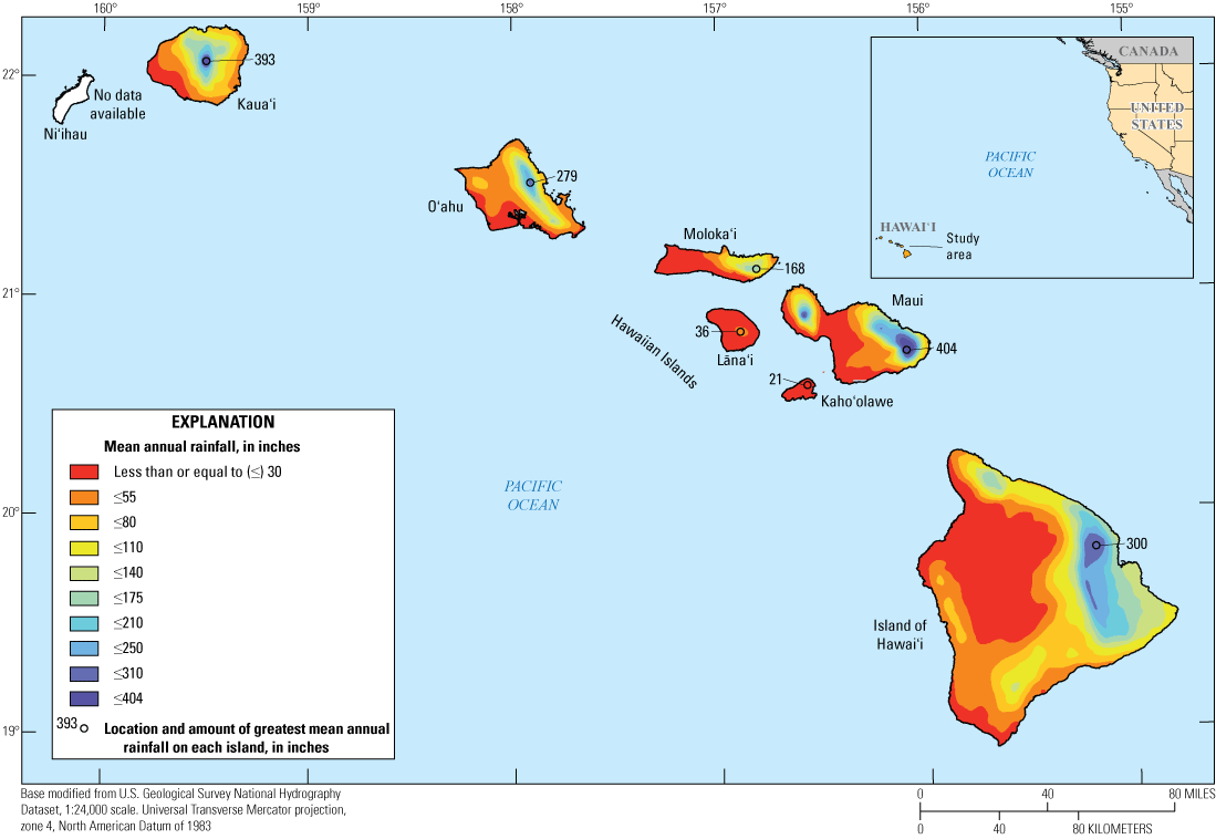
Distribution of mean annual rainfall, State of Hawaiʻi (modified from Giambelluca and others, 2013), 1911–2020.
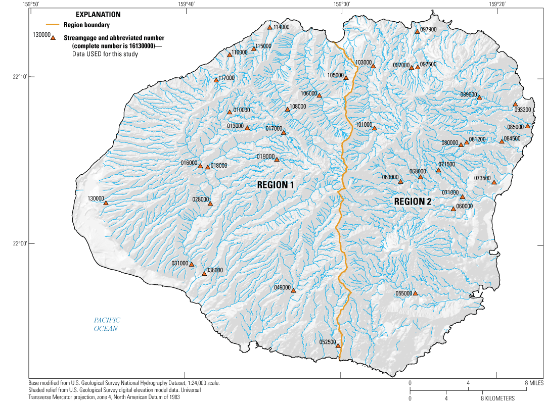
Streamgages with at least 10 years of usable peak-flow data, Kauaʻi, State of Hawaiʻi, 1911–2020.
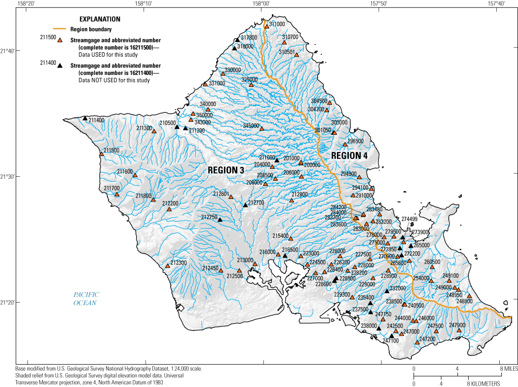
Streamgages with at least 10 years of usable peak-flow data, Oʻahu, State of Hawaiʻi, 1911–2020.
Streamgages with at least 10 years of usable peak-flow data, Molokaʻi, State of Hawaiʻi, 1911–2020.
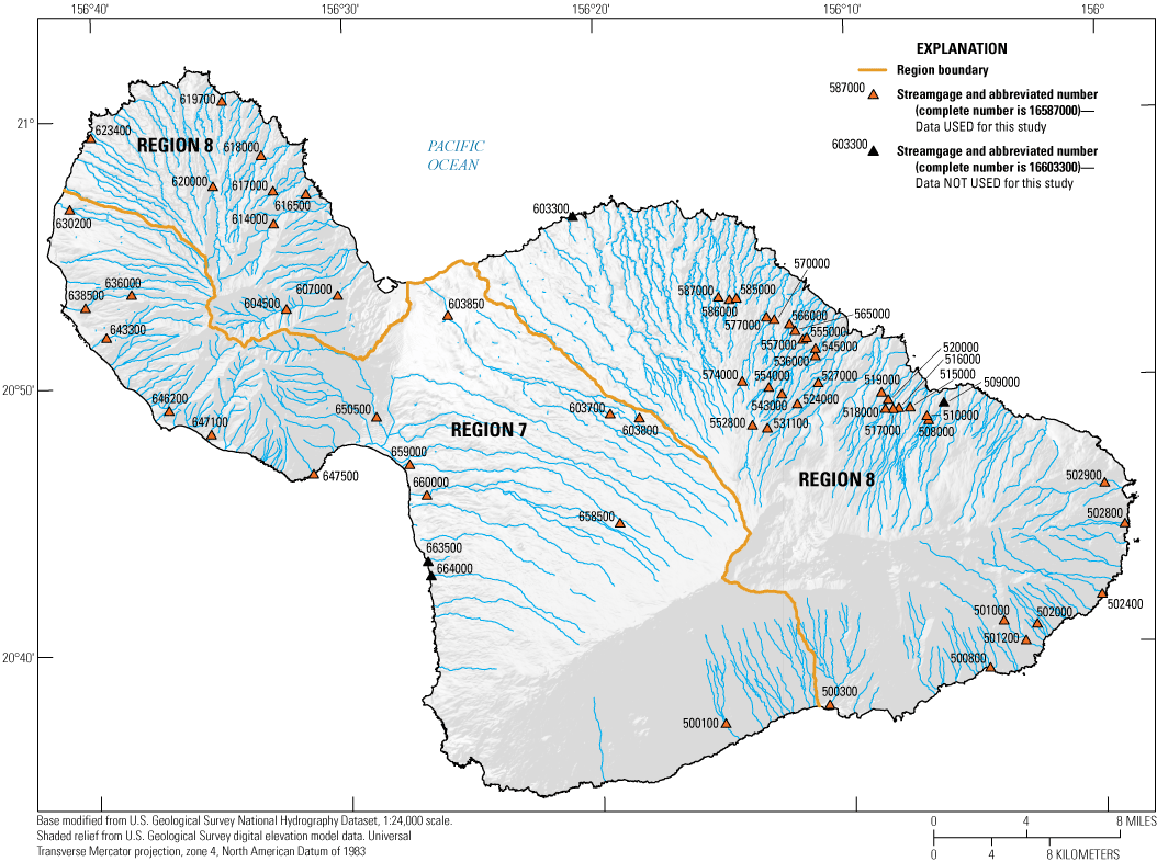
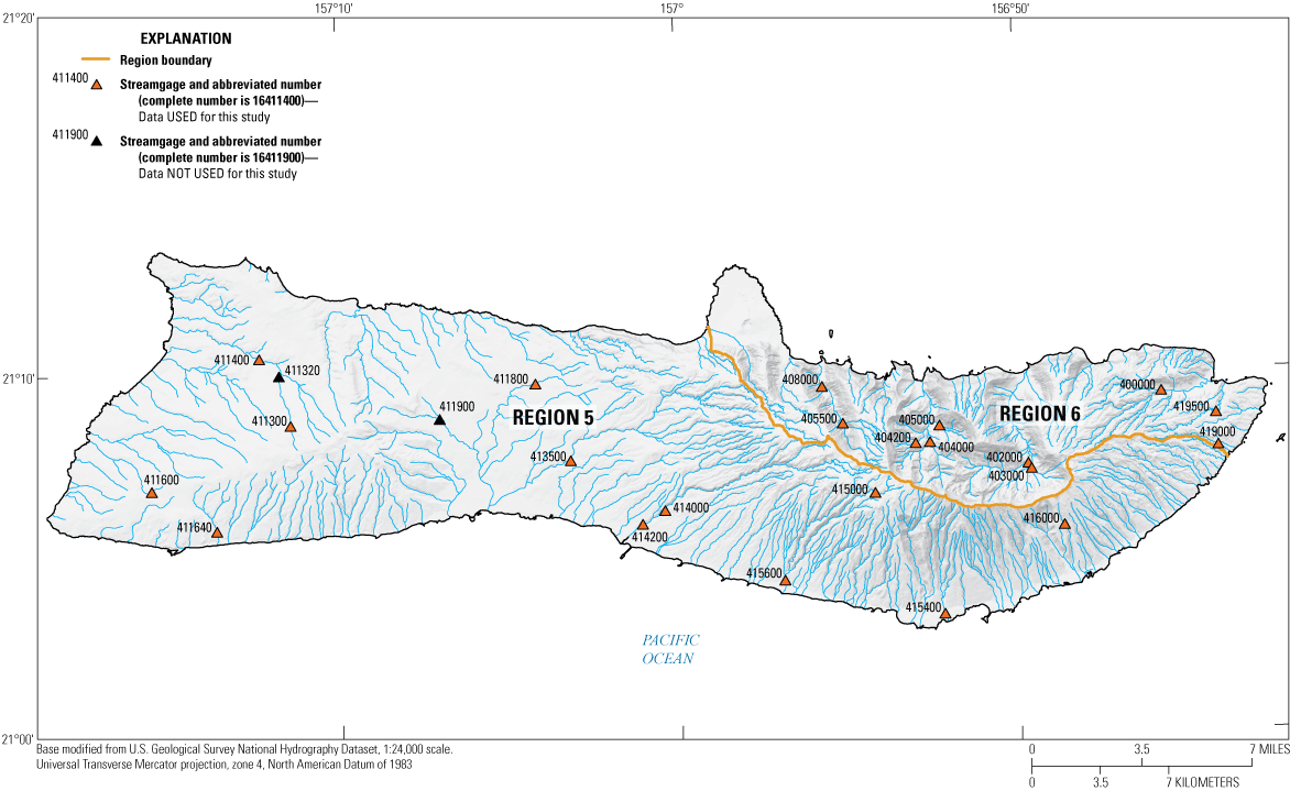
Streamgages with at least 10 years of usable peak-flow data, Maui, State of Hawaiʻi, 1911–2020.
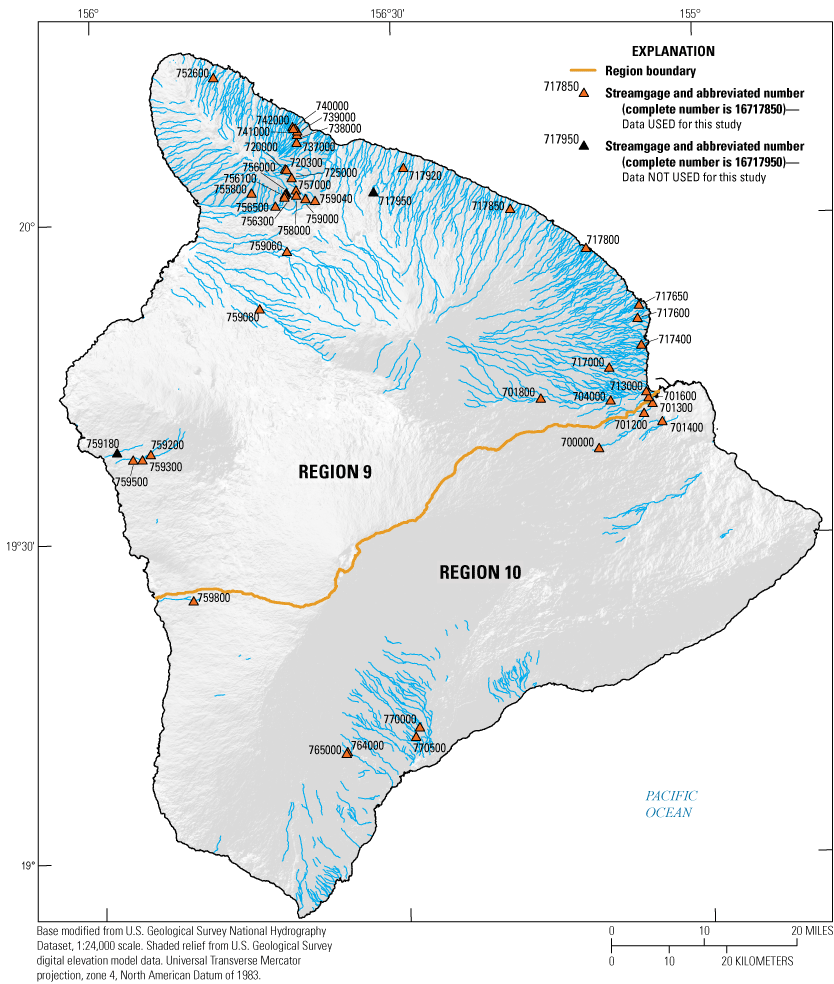
Streamgages with at least 10 years of usable peak-flow data, Island of Hawaiʻi, State of Hawaiʻi, 1874–2007.
Purpose and Scope
The purpose of this report is to present methods and results for estimating the magnitude and frequency of floods for unregulated streams on five of the main Hawaiian Islands: Kauaʻi, Oʻahu, Molokaʻi, Maui, and Hawaiʻi. (Unregulated streams are those for which peak flows are not altered to a large extent by upstream reservoirs, dams, diversions, or other structures.) The report describes (1) updated flood flows at selected streamgages for the 50-, 20-, 10-, 4-, 2-, 1-, 0.5-, and 0.2-percent AEPs using peak-flow data through water year 2020, (2) regional-skew estimates for Hawaiʻi, (3) regression equations for relating basin and climatic characteristics to flood flows at ungaged stream sites for the 50-, 20-, 10-, 4-, 2-, 1-, 0.5-, and 0.2-percent AEPs, and (4) the accuracy and limitations of the regression equations. The regression equations developed were incorporated in the web-based USGS StreamStats application for Hawaiʻi (Rosa and Oki, 2010). This report supersedes previous flood-frequency reports in Hawaiʻi (the most recent being Oki and others, 2010) by including more recent peak-flow data through water year 2020 (table 2) and by implementing advances in statistical techniques developed after previous reports were published.
Table 2.
Comparison of annual peak-flow data used in this study through water year 2020 relative to data used in a previous U.S. Geological Survey flood-frequency study (Oki and others, 2010), State of Hawaiʻi.Previous Studies
The USGS began collecting streamflow data in Hawaiʻi in 1909 (Yamanaga, 1972, p. 1). The number of active streamgages increased until the late 1960s and decreased steadily since that time. In water year 2020, the USGS had 137 active streamgages in Hawaiʻi (the number of active streamgages includes streamgages that are not included in the present study).
Previous flood studies in Hawaiʻi include descriptive and quantitative investigations related to storm-drainage standards, peak-flow statistics, and (or) regional regression equations at spatial scales ranging from individual floods to statewide studies. For a detailed list and descriptions of past studies related to floods in Hawaiʻi, see Oki and others (2010, app. A). Prior to the study described in this report, the most recent estimates of peak-flow statistics for streams in Hawaiʻi were published in 2010 (Oki and others, 2010), using data from streamgages on Kauaʻi, Oʻahu, Molokaʻi, Maui, and Hawaiʻi through water year 2008. Oki and others (2010) applied the methods described in Bulletin 17B (Interagency Advisory Committee on Water Data, 1982) to estimate AEP flows at 235 streamgages and developed regression equations to relate flood flows to basin characteristics at ungaged locations. Peak-flow estimates from Oki and others (2010) are compared to those generated by this study in the “Comparison of Results with Previous Studies” section.
Description of Study Area
The eight main islands in the State of Hawaiʻi, located in the north Pacific Ocean, trend northwest to southeast and have a total land area of 6,420 square miles (mi2). The majority of each island was formed by shield-stage volcanic eruptions, and the southeastern islands are geologically the youngest. The area considered for flood-frequency analysis in this study (hereinafter referred to as “study area”) includes the five islands of Kauaʻi, Oʻahu, Molokaʻi, Maui, and Hawaiʻi, which have a total land area of 5,904 mi2. The maximum altitudes for the islands in the study area are 5,246 feet (ft) for Kauaʻi; 4,046 ft for Oʻahu; 4,948 ft for Molokaʻi; 10,016 ft for Maui; and 13,781 ft for Hawaiʻi (U.S. Geological Survey, 2013). The individual islands in the study area are commonly divided into two physiographic zones, windward and leeward, based on their exposure to the predominant northeasterly winds.
Drainage basins in the study area are characterized by relatively small sizes, amphitheater-shaped valley heads, steep walls, and gently sloping floors (Wong, 1994). In geologically older areas (for example, northern Kauaʻi) with abundant rainfall, erosion and mass wasting have created large valleys and well-defined stream channels; in geologically younger areas (for example, southern Island of Hawaiʻi), valleys are smaller and well-defined stream channels are uncommon because high-permeability soils and rocks at the surface allow rainwater to infiltrate before eroding the land. The topography of Hawaiian shield volcanoes leads to a radial drainage pattern where streams tend to flow away from each other (Oki and others, 2010).
Climate
The climate of Hawaiʻi is characterized by mild temperatures, moderate humidity, prevailing northeasterly winds, a dry summer season from May through September, and a wet winter season from October through April (Sanderson, 1993). Hawaiʻi lies to the southwest of the North Pacific anticyclone—a semi-permanent, high-pressure atmospheric system that is responsible for the prevailing northeasterly winds, known locally as “trade winds” (Wyrtki and Meyers, 1976). The North Pacific anticyclone and other migratory weather systems are the dominant controls on Hawaiʻi’s climate (Schroeder, 1981; Lyons, 1982; Chu and others, 1993). During the dry season, the trade winds blow 85 to 95 percent of the time (Sanderson, 1993; Garza and others, 2012). During the wet season, the trade winds diminish (only blowing 50–80 percent of the time), which allows more migratory storm systems to influence the islands’ weather.
Rainfall
Rainfall in Hawaiʻi has extreme spatial gradients related to altitude and the orientation of the topography relative to the northeasterly trade winds (Giambelluca and others, 1986; Sanderson, 1993) (fig. 6). As moist air from the northeast encounters the windward slopes of the islands, the air rises, cools, and condenses to form precipitation known as “orographic rainfall.” The air that passes over the windward slopes loses moisture, resulting in substantially less rainfall for the areas on the leeward (southwest) side of mountain barriers—this is known as the “rain-shadow effect” (Giambelluca and others, 1986). In some places, mean annual rainfall can vary by as much as 100 inches per mile (Giambelluca and others, 2013). Rainfall maxima for the islands in the study area are 393 inches per year (in/yr) for Kauaʻi, 279 in/yr for Oʻahu, 168 in/yr for Molokaʻi, 404 in/yr for Maui, and 300 in/yr for Hawaiʻi (Giambelluca and others, 2013). Rainfall maxima for each island generally occur on the windward slopes between altitudes of 2,000 and 6,000 ft (Giambelluca and others, 2013). Precipitation decreases above altitudes of 6,000 ft because of a trade wind inversion, where moist air is prevented from continuing to rise up the mountain because air temperatures increase with altitude between about 6,000 and 8,000 ft (Giambelluca and Nullet, 1991; Chen and Feng, 1995; Cao and others, 2007).
Rain gages across Hawaiʻi hold many of the United States records for extreme rainfall, including the 24-hour record set in 2018 when 49.7 inches of rain fell at Waipā Garden near Hanalei, Kauaʻi (National Oceanic and Atmospheric Administration, 2018). Although trade-wind-driven orographic rainfall contributes the majority of the annual rainfall for most areas, rainfall associated with atmospheric disturbances may be responsible for most of the high-intensity rainfall events (Longman and others, 2021). Intense rainfall in Hawaiʻi is usually related to one of the following four types of atmospheric disturbances:
-
(1) cold fronts;
-
(2) subtropical cyclones (Kona lows);
-
(3) upper-tropospheric disturbances (upper-level lows); and
-
(4) tropical cyclones (Kodama and Barnes, 1997; Caruso and Businger, 2006; Perica and others, 2009; Longman and others, 2021).
El Niño-Southern Oscillation, Pacific Decadal Oscillation, and the Pacific North American
Three natural teleconnections (related climate anomalies that are separated by large distances) exert strong influences on the climate of Hawaiʻi: El Niño–Southern Oscillation (ENSO), Pacific Decadal Oscillation (PDO), and the Pacific North American (PNA). These teleconnections, which operate on different time scales, are not independent and in some cases can modulate the effects of each other (Chu and Chen, 2005; Yu and Zwiers, 2007; Frazier and others, 2018).
One of the primary drivers behind interannual climate variability for Hawaiʻi is ENSO (Lyons, 1982; Chu, 1995; Chu and Chen, 2005; Elison Timm and others, 2011), which characterizes the combined effects of sea-surface-temperature and atmospheric-pressure anomalies in the tropical Pacific Ocean (Rasmusson and Carpenter, 1982; Trenberth, 1997). The ENSO cycle is commonly divided into three phases based on sea-surface-temperature anomalies in the central and eastern tropical Pacific Ocean: El Niño (warm ocean water), La Niña (cold ocean water), and neutral. ENSO phases generally last 6–18 months and can have wide-ranging effects on rainfall, surface-air temperatures, and global-circulation patterns (Trenberth and Hurrell, 1994; Kestin and others, 1998; Kim and others, 2003). Generally, El Niño phases result in below-average rainfall and La Niña phases result in above-average rainfall for Hawaiʻi (Ropelewski and Halpert, 1987; Chu, 1995; Chu and Chen, 2005; Giambelluca and others, 2013); however, rainfall during La Niña phases may have started to decrease in the early 1980s (O’Connor and others, 2015). In addition to the generally positive correlation between La Niña phases and annual rainfall, extreme rainfall events may be more likely during La Niña phases than El Niño phases (Chu and others, 2010; Chen and Chu, 2014).
The PDO has similar characteristics to ENSO but operates on an interdecadal time scale: PDO phases last about 20–30 years (Mantua and others, 1997; Minobe and Mantua, 1999). The PDO index, the most common metric of the PDO, is the leading principal component of an empirical orthogonal function analysis of sea-surface-temperature anomalies over the North Pacific Ocean (poleward of 20°N) (Mantua and Hare, 2002). Positive phases of the PDO index are associated with cooler water in the interior of the North Pacific Ocean and warmer water along the Pacific coast of North America; the opposite pattern occurs during the negative phase (Mantua and others, 1997). Rainfall in Hawaiʻi is negatively correlated with the PDO index (Mantua and others, 1997; Chu and Chen, 2005; Diaz and Giambelluca, 2012), and positive PDO phases may strengthen the effects of ENSO variability on rainfall (Chu and Chen, 2005; Verdon and Franks, 2006; Elison Timm and others, 2020). The PDO index shifted from a positive phase into a predominantly neutral or negative phase during the 1990s and returned to a positive phase in about 2014 (National Oceanic and Atmospheric Administration, 2021).
The PNA teleconnection relates the atmospheric circulation pattern over the North Pacific with the pattern over North America (Wallace and Gutzler, 1981; Leathers and others, 1991). The PNA—which has both a positive and negative phase—is quasi-periodic and has a recurrence interval ranging from a few years to a few decades (Wallace and Gutzler, 1981; Trouet and Taylor, 2010). During the positive phase, Hawaiʻi tends to receive less rainfall; during the negative phase, Hawaiʻi tends to receive more rainfall (Chu and others, 1993). Jayawardena and Chen (2016) found that a negative PNA phase was associated with three unusually prolonged heavy-rainfall periods in 1951, 1979, and 2006. In a multiple-linear regression analysis using ENSO, PDO, and PNA to model rainfall in Hawaiʻi, Frazier and others (2018) determined that PNA best describes the interannual variability in wet-season rainfall, whereas ENSO best describes the interannual variability in dry-season rainfall. (Frazier and others [2018] defined the wet season and dry season as November–April and May–October, respectively.)
Trends in Extreme Rainfall
Global climate change and cyclical changes in regional climate may influence the frequency and intensity of heavy rainfall events in Hawaiʻi. Studies of past rainfall extremes—using daily rainfall data, annual maximum daily rainfall data, and climate-change indices—have found generally decreasing trends for Oʻahu, Maui, and Kauaʻi (Kruk and Levinson, 2008; Perica and others, 2009; Chu and others, 2010; Elison Timm and others, 2011; Chen and Chu, 2014; Huang and others, 2021). For most measures of extreme rainfall, the Island of Hawaiʻi was the only island in the study area that had some evidence of increasing trends (Chu and others, 2010; Chen and Chu, 2014); however, Huang and others (2021) reviewed daily rainfall maxima during 1970–2005 and found no evidence of consistent increases on the Island of Hawaiʻi. Analyses of extreme rainfall trends on Molokaʻi are inconclusive due to limited historical data. Causes for the generally decreasing trends are uncertain but may be related to a poleward shift in the Pacific storm track (Yin, 2005), the increasing frequency and decreasing altitude of the trade-wind inversion (Cao and others, 2007; Longman and others, 2015), or decreasing in trade-wind frequency (Garza and others, 2012). The factors affecting rainfall climatology in Hawaiʻi are complex, and estimates of future trends in extreme rainfall remain inconclusive (Elison Timm and others, 2011; Norton and others, 2011; Elison Timm and others, 2020; Xue and others, 2020).
Flood Characteristics
Streamflow in Hawaiʻi consists of the following:
-
(1) direct runoff of rainfall, in the form of overland flow and subsurface stormflow that rapidly returns infiltrated water to the stream;
-
(2) groundwater discharge, in the form of base flow, where the stream intersects the water table;
-
(3) water returned from stream-bank storage;
-
(4) rain that falls directly on streams; and
-
(5) any additional water, including excess irrigation water discharged to the stream by humans (Oki, 2003).
In heavy rainfall leading to most floods, direct runoff is the primary contributor to streamflow. Variables that affect flood magnitude for a given watershed include rainfall intensity and duration, antecedent soil moisture, soil permeability, depth to the water table, and available surface-depression storage (Ivancic and Shaw, 2015; Wasko and Sharma, 2017; Wasko and Nathan, 2019). Huang and others (2021) examined annual maxima from paired streamgages and rainfall gages in the same or similar watersheds in Hawaiʻi during 1970–2005 and found that the streamflow and rainfall maxima rarely occurred on the same dates, reinforcing the concept that daily rainfall totals are not the only factor governing flood magnitude (Sharma and others, 2018).
Floods can occur during any time of the year in Hawaiʻi but are most common during the rainy season (October–April) when atypical storms and wind patterns replace the predominant northeasterly trade winds. Streams on the leeward sides of mountain ridges may be dry for most of the year, only to be punctuated by a few floods from large storms. Streams on the windward sides of mountain ridges may flow perennially because of persistent trade-wind-driven rainfall and groundwater discharge as base flow. Seasonal differences in streamflow are most pronounced for the leeward-facing streams.
Streams in Hawaiʻi tend to be flashy—that is, they respond quickly to rainfall and have short-lived discharge peaks—because of small and steep drainage basins and high-intensity rainfall from storms (Wong, 1994). Flood hydrographs generally have a characteristic steep triangular shape, indicating a rapid rise and fall in discharge (Wu, 1969). Stream stage will commonly rise and fall several feet over a few hours in response to intense rainfall. In some floods, stream discharge can change by a factor of 60 in 15 minutes (Tomlinson and De Carlo, 2003).
Land Cover
Land cover in Hawaiʻi—representing the physical condition of the land, rather than how the land is used—varies temporally and spatially. The general trend from the early 1900s to 2020 was an increase in population and urbanization and a decrease in large-scale agriculture. The population of the State of Hawaiʻi increased from 154,001 in 1900 to 1,455,271 in 2020 (U.S. Census Bureau, 2021). Agriculture—mostly pineapple and sugar cane—was the dominant industry in Hawaiʻi during the early 1900s, peaked in the 1920s with about 391 square miles of cropland for the islands in the study area, and began to decline in the 1950s (Water Resource Associates, 2003; Suryanata, 2009). In nominal 2011 conditions, crops covered no more than 10 percent of the land on any island in the study area, for a total of about 190 square miles: Maui had the highest percent of cropland (9.6 percent), and Molokaʻi had the lowest percent of cropland (1.8 percent) (National Oceanic and Atmospheric Administration, 2014). Nominal 2011 land-cover data for Hawaiʻi are separated into 18 classes and are available at a 2.4-meter resolution (National Oceanic and Atmospheric Administration, 2014).
As population increased and large-scale agriculture decreased, the degree of urbanization increased. Urbanization tends to increase flood magnitude because built, impervious surfaces prevent water from infiltrating the soil, resulting in a greater fraction of rainfall that contributes to overland flow and stream discharge (Hollis, 1975; Schueler, 1994; Konrad, 2003). The percentage of impervious land cover is a common metric of urbanization that can be easily and accurately quantified with remote sensing (Weng, 2012; National Oceanic and Atmospheric Administration, 2014). Impervious surfaces associated with urbanization include roofs, paved roads, and parking lots. The relative effects of impervious surfaces on flood magnitude generally decrease as the flood magnitude increases; that is, the magnitude of floods with high AEPs (small floods) is affected more by changes in impervious land cover in the drainage basin than is the magnitude of floods with low AEPs (large floods) (Hollis, 1975; Terstriep and others, 1976; Dudley and others, 2001). The islands in the study area have the following percentage of their land cover classified as impervious: Kauaʻi, 2.8 percent; Oʻahu, 14.5 percent; Molokaʻi, 1.1 percent; Maui, 3.3 percent; Hawaiʻi, 1.2 percent (National Oceanic and Atmospheric Administration, 2014). Beyond the direct effects of impervious surfaces, urbanization can affect flood magnitude and frequency by compacting soils and decreasing infiltration capacity, fragmenting and draining wetlands, reducing floodplain sizes, and channelizing stream reaches (Murabayashi and Fok, 1979; Dudley and others, 2001; Shuster and others, 2005).
Data Collection and Compilation
Available peak-flow data from USGS streamgages in Hawaiʻi were screened for suitability in flood-frequency analysis. Selection considerations included record length, the effects of regulations or diversions, and the amount of impervious land cover in the drainage basin. Peak-flow data from the selected sites were then reviewed to ensure data quality and evaluated for the presence of trends. After selecting the streamgages and reviewing the peak-flow data, a suite of basin and climatic characteristics was determined for each streamgage and associated drainage basin for use in the development of regression equations.
Streamgage Selection and Peak-Flow Data
Peak-flow data for streamgages with at least 10 years of record were downloaded from the USGS National Water Information System (NWIS; https://waterdata.usgs.gov/nwis) database (U.S. Geological Survey, 2021); flood-frequency analyses at a streamgage with less than 10 years of record are generally unreliable (England and others, 2019, p. 36). Data through water year 2020 were used at all streamgages where available. At the time of analysis, USGS streamgages 16103000 (Hanalei River near Hanalei, Kauaʻi) and 16325000 (Kamananui Stream at Pupukea Mil Road Oʻahu) did not have approved 2020 peaks. Additionally, 2021 peaks for USGS streamgages 16345000 (Opaeula Stream near Wahiawa, Oʻahu) and 16587000 (Honopou Stream near Huelo, Maui) were included in the analysis because they were the largest floods on record for each streamgage. Streamgages in Hawaiʻi typically are either continuous-record gages or crest-stage gages. Continuous-record gages record the stage (height) of streamflow at short intervals (for example, every 15 minutes, although the recording interval may be automatically decreased during times of rapidly changing flow at higher stages), whereas crest-stage gages record only the maximum stage of floods above a certain threshold. Discharge is computed from stage measurements at streamgages using a site-specific stage-discharge relation or indirect-measurement methods.
Initially, 268 active and discontinued streamgages were identified as potential streamgages to include in the flood-frequency analysis. The number of usable streamgages was reduced to 238 after reviewing the data (figs. 2–6; table 1.1, app. 1). Streamgages with fewer than 10 years of usable peak-flow data were excluded (including some streamgages where peaks were removed in a low-outlier screening that will be described in section, “Low Outliers Identified with the Multiple Grubbs-Beck Test”). Five streamgages with regulated or diverted flow (NWIS qualification code 6) were excluded (table 1.2, app. 1). Streamgages where discharge was affected to an unknown degree by regulation or diversion (NWIS qualification code 5) were retained except for USGS streamgage 16210500 (Kaukonahua Stream at Waialua, Oʻahu), which was excluded because peak flows may have been substantially affected by regulation. Streamgages with drainage basins that had impervious surfaces covering more than 20 percent of the land were excluded because of the potential effects of impervious surfaces and urbanization on peak flows (see section, “Land Cover”). (The exclusion criterion for urbanized streamgages in the current study—greater than 20 percent impervious surface in the drainage basin—is about equal to the exclusion criterion used by Oki and others (2010) for the 238 streamgages in the current study: greater than 20 percent combined medium- and high-intensity development in the drainage basin.) Additionally, data from 18 streamgages were excluded because of possibly inaccurate rating curves or other potential issues (R.A. Fontaine, U.S. Geological Survey, written commun., 2020). Streamgages and data excluded from the analysis are available in appendix 1 (table 1.2).
From the 238 streamgages used in the study, the average number of available annual peaks for each streamgage is 40. The longest available record, 109 annual peaks, is from Honopou Stream on Maui (USGS streamgage 16587000). The number of available annual peaks for this study reached a maximum of 169 peaks in 1967–68 and has steadily decreased since (fig. 7). About 81 percent of annual peak used in this study with known dates occurred during the wet season from October to April (fig. 8).
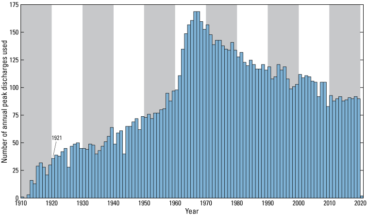
Total number of annual peak discharges used for each year in this study, State of Hawaiʻi, 1911–2021.
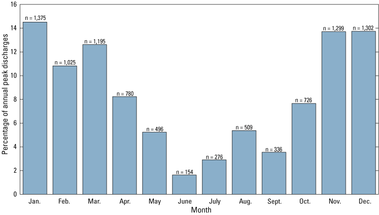
Percentage of annual peak discharges by month for this study, State of Hawaiʻi, 1911–2021. The number of annual peak discharges (n) in each month is shown on the top of each bar. Annual peak discharges with unknown months are excluded.
This study includes 18 streamgages that were not used by Oki and others (2010)—the most recent flood-frequency study for Hawaiʻi—and excludes 15 streamgages that were used by Oki and others (2010) (tables 1.2 and 1.3, app. 1). Most of the newly included streamgages had fewer than 10 usable annual peaks in 2010; most of the newly excluded streamgages were omitted because they had fewer than 10 usable annual peaks after screening for low outliers.
Trends in Peak Flows
The Bulletin 17C methods for flood-frequency analysis (England and others, 2019) used in this study assume that (1) the peak-flow data are a random, independent, and identically distributed sample that is representative of the population of floods, and (2) the parameters describing the statistical distribution of floods will not change in the future (that is, the distribution is stationary). These assumptions may be violated by deterministic trends related to abrupt or gradual changes in stream regulation, land cover and land use, or climate, or a mixture of those sources (Milly and others, 2008; Vogel and others, 2011). Stationarity can be difficult to detect in hydrologic time series, however, because natural processes often exhibit low-frequency deviations that persist for decades or centuries (Cohn and Lins, 2005; Villarini and others, 2009; Lins and Cohn, 2011). To evaluate the assumptions of the Bulletin 17C methods, peak-flow data were tested for monotonic trends and step trends. Trends were considered statistically significant for probability values (p-values) less than or equal to 0.05—this is the probability that an observed trend is due to random chance.
Methods for Trend Analyses
To prepare the peak-flow data for trend testing, the censored values—peaks reported as below or above a threshold, rather than a discrete peak—were temporarily modified. Failure to account for censored data when conducting statistical analyses can result in inaccurate conclusions because censored data (for example, less than [<] 80 ft3/s) represent different information than discrete data (for example, 80 ft3/s). The peak-flow data in the current study contain 274 left-censored peaks (about 3 percent of the total peaks), which indicate that the annual peak flood was below a certain discharge, and only two right-censored peaks (about 0.02 percent of the total peaks), which indicate that the annual peak flood was above a certain discharge. Left-censored peaks occur when all flood flows during a year are below the minimum recordable discharge at a streamgage and the exact peak discharge is unknown. For the 57 streamgages with at least 1 left-censored peak, each peak less than the largest left-censored peak was replaced with the largest left-censored peak (Helsel, 2012, p. 14; Helsel and others, 2020, p. 357). For example, if the record for a streamgage contains annual peak discharges of <400, 300, 600, <100, and 700 ft3/s, then the record would be recoded to <400, <400, 600, <400, and 700 ft3/s. Although recoding the values results in a loss of information, significant trends found with the recoded data are more believable (Helsel and others, 2020, p. 357). The records containing recoded values were only used for trend analyses and the unaltered records were used for the remainder of the flood-frequency analysis. The two right-censored peaks (at USGS streamgages 16502900 [Kawaipapa Gulch at Hana, Maui] and 16604500 [Wailuku River at Kepaniwai Park, Maui]) were not modified and were treated as discrete peaks.
Monotonic trends in peak-flow data, representing a unidirectional change over time, were evaluated using the nonparametric Mann-Kendall test (Helsel and others, 2020, p. 332). Three versions of the Mann-Kendall test with different dependence assumptions were applied using scripts written in the R coding language (R Core Team, 2021) by Dudley and others (2018). The dependence assumptions relate to autocorrelation (also known as “serial correlation”), which describes the tendency for years with high peak flows to be followed by years with high peak flows and for years with low peak flows to be followed by years with low peak flows (Helsel and others, 2020, p. 5). The first version, the standard Mann-Kendall test, assumes the annual peaks are independent of each other with time. The second version, adapted from Hamed and Rao (1998), assumes that the annual peaks have short-term persistence (STP; or lag-one autocorrelation); that is, the autocorrelation decays exponentially or faster as the time lag increases. The third version, adapted from Hamed (2008), assumes that the annual peaks have long-term persistence (LTP); that is, the autocorrelation decays slower than exponentially as the time lag increases (Koutsoyiannis and Montanari, 2007). LTP is characterized by quasi-periodic excursions in the central tendency of a variable (Helsel and others, 2020, p. 359) and is likely present in most natural hydroclimatological systems (Koutsoyiannis and Montanari, 2007; Lins and Cohn, 2011). In many cases, LTP is indistinguishable from a deterministic trend because a trend may simply be one limb of an LTP-driven oscillation, particularly for data with relatively short records (Villarini and others, 2009). The presence of persistence (either STP or LTP) does not inherently violate the assumption of stationarity; however, persistence may result in an overestimation of the significance of trends determined from tests that assume independence of the data (Cohn and Lins, 2005; Helsel and others, 2020, p. 359). The use of a modified trend test that accounts for persistence results in only a very small loss of power, even if the data possess no persistence (Cohn and Lins, 2005).
Step trends, also called “change points,” are abrupt shifts in the statistical properties of time-series data (Reeves and others, 2007; Helsel and others, 2020, p. 352). For peak-flow data, step trends may be related to changes in flood regulation, climate, land use, or land cover. Change points in the peak-flow data were analyzed using the Pettitt test (Pettitt, 1979)—a derivative of the nonparametric Mann-Whitney two-sample test—to determine the optimum point to split each time series into two (Ryberg and others, 2020). Although multiple change points may exist in a record, the Pettitt test is limited to identifying a single change point. The Pettitt test does not account for temporal gaps in the record and assumes that all data are equally spaced. The accuracy of results from the Pettitt test may be affected by autocorrelation and monotonic trends (Busuioc and Storch, 1996); however, a change-point test that accounts for autocorrelation was unavailable. Differentiating between step trends and monotonic trends can be difficult, especially for short records—the two trend types should be analyzed together to develop a more complete understanding of the data (McCabe and Wolock, 2002; Sharma and others, 2016).
Peak-Flow Trend Results
Statistically significant monotonic trends were detected at 51 of the 238 streamgages used in this study for at least one of the Mann-Kendall trend-test versions (app. 2). Under the independence assumption, 29 streamgages had decreasing trends and 18 streamgages had increasing trends; under the STP assumption, 26 streamgages had decreasing trends and 16 streamgages had increasing trends; and under the LTP assumption, 6 streamgages had decreasing trends and 4 streamgages had increasing trends. Of the 90 active streamgages (those with annual peaks reported for water year 2020), 24 have significant trends: 16 decreasing and 8 increasing. Of the streamgages with significant monotonic trends, streamgages on Kauaʻi, Oʻahu, and the Island of Hawaiʻi had predominantly decreasing trends, whereas streamgages on Maui and Molokaʻi had mixed results. The magnitude of the trend during the record period at each streamgage was estimated using the Theil slope (also known as the Kendall-Theil robust line) (Helsel and others, 2020, p. 332) (app. 2).
The results from trend testing should be reviewed in the context of spatial and temporal data availability. Test results depend considerably upon the time period analyzed: the available peak-flow data sometimes represent neither long nor concurrent record periods (fig. 9).
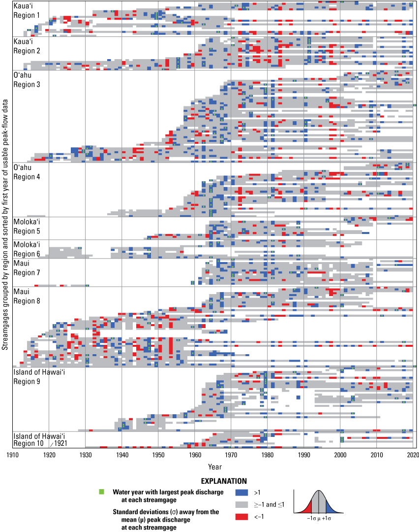
Temporal availability of peak-flow data for each region and island in the study area, State of Hawaiʻi. Streamgages are grouped into regions and sorted by the first year of usable peak-flow data, 1911–2021. The color for each water year represents the magnitude of the peak discharge, in standard deviations away from the mean at each streamgage. Symbols: >, greater than; ≥, greater than or equal to; ≤, less than or equal to; <, less than.
In some cases, short-term trends related to natural climate variability can be superimposed on long-term deterministic trends. A flag plot was created by applying the Mann-Kendall trend test (with the independence assumption) to all possible pairs of starting and ending years (minimum 10 annual peak discharges) for each streamgage to determine the percentage of streamgages with statistically significant increasing and decreasing trends for various periods (fig. 10). Record periods ending before about 1980 had predominantly increasing trends; record periods ending after about 1980 had predominantly decreasing trends. Additionally, decadal trends in peak flows were analyzed by applying the Mann-Kendall trend test (with the independence assumption) to each record subperiod spanning 10 years (for example, 1975–84) and containing at least eight annual peaks. The results are shown in figure 11, where the values represent percentages of streamgages with increasing or decreasing trends for the decade, plotted on the mid-decade year (for example, for 1975–84, the mid-decade year would be 1979). Increasing peak-flow trends were common during the decades centered around 1946–48, 1963–64, 1987–88, 2001–03, and 2013–14. Decreasing peak-flow trends were common during the decades centered around 1968–73 and 1993–96.
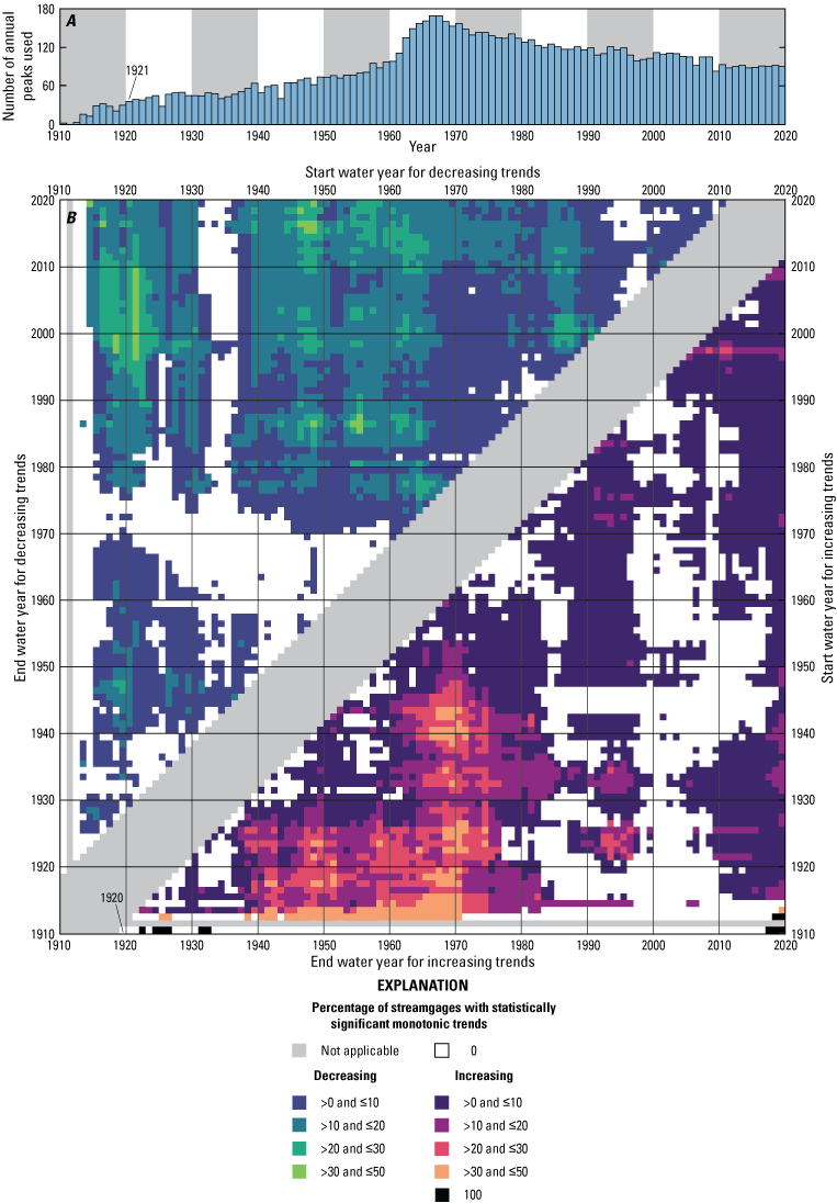
Number of annual peaks used for each year in the study (A) and a flag plot showing the percentage of streamgages with statistically significant increasing and decreasing monotonic trends in annual peak discharge (B), State of Hawaiʻi, 1911–2020. Significant trends were determined using the Mann-Kendall trend test under the independence assumption with a probability value (p-value) of 0.05. Symbols: >, greater than; ≤, less than or equal to.
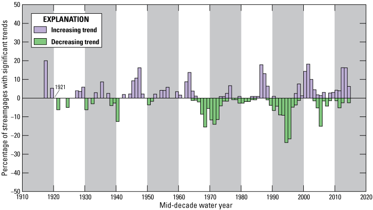
Percentage of streamgages with statistically significant decadal trends in annual peak discharge, State of Hawaiʻi, 1915–2015. The percentage of significant trends is plotted on the mid-decade water year (for example, for 1975–84, the mid-decade year would be 1979). Significant trends were determined using the Mann-Kendall trend test under the independence assumption with a probability value (p-value) of 0.05.
Significant step trends in peak-flow data were found at 44 streamgages (fig. 12; app. 2). Twenty-six streamgages with significant step trends had peak-flow magnitudes that decreased after the change point; 18 streamgages had peak-flow magnitudes that increased after the change point. Decreasing step trends most commonly have change points clustered from the 1970s to the early 2000s, whereas increasing step trends have a broad distribution of change points spanning the 1930s to 2000s. As with monotonic trends, comparisons of step trends and change points between streamgages should be made with caution because of sometimes inconsistent record periods available for analysis (fig. 9). One of the clearest patterns is that, of the 20 streamgages with statistically significant step trends on Oʻahu, 11 have change points during 1968–76.
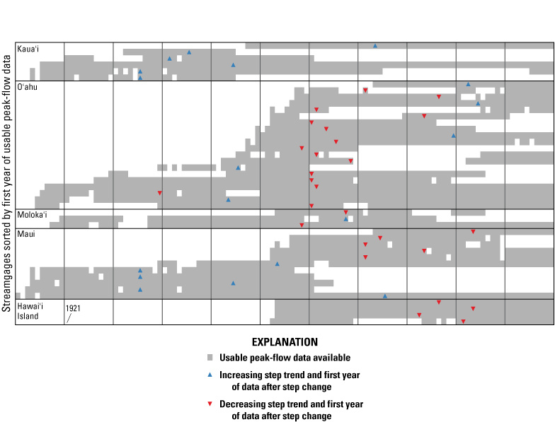
Results of the Pettitt test for step trends applied to peak-flow data from streamgages used in this study, State of Hawaiʻi, 1911–2020. Only streamgages with statistically significant trends (p-values ≤ 0.05) are shown. Streamgages are grouped into islands and sorted by the first year of usable peak-flow data. The first year following the step change is indicated by a triangle.
Time-series data can possess both monotonic trends and step trends, or one type of trend may mask the other. Thirty-four streamgages had a significant monotonic trend (using the independence assumption) and a significant step trend. Further evaluations of trends in the peak-flow data may consider analyzing the time periods before and after significant change points separately and (or) applying adjustments to the data to account for autocorrelation before using the Pettitt test for step trends.
In summary, trend analyses of the peak-flow data used in this study suggest that decreasing trends are more common than increasing trends. For monotonic trends, the number of significant trends decreases when STP and LTP are accounted for. Monotonic and step trend tests suggest that peak-flow magnitude has generally decreased since about 1980, although the number of streamgages with significant trends may be overestimated by the presence of natural hydroclimatologic fluctuations related to LTP.
Stationarity should be the default assumption for flood-frequency analyses, unless the nonstationarity assumption can be justified based on a clear understanding of the physical processes of trends (Lins and Cohn, 2011; Serinaldi and Kilsby, 2015; Salas and others, 2018; England and others, 2019; Ryberg and others, 2020). Although this study presents a cursory summary of peak-flow trends at streamgages, an exhaustive investigation of trends and the potential causes of trends is beyond the scope of this report. If additional data and more comprehensive analyses discover relations not discussed here, future flood-frequency analyses may consider incorporating trends and nonstationarities and (or) excluding stations with definitive nonstationarities related to deterministic trends. In the absence of clear relations between trends and hydroclimatological forcings, the assumptions in Bulletin 17C (England and others, 2019) are presumed to be valid and are retained for this study.
Physical and Climatic Basin Characteristics
Drainage basins for each streamgage used in the study were delineated using geographic information system (GIS) methods. Physical and climatic basin characteristics for each streamgage were estimated using available datasets. Accurate basin delineations and basin characteristics are critical for the regional regression analysis relating basin characteristics to flood discharges. The source data used to determine the basin delineations and basin characteristics were incorporated into the USGS StreamStats application for Hawaiʻi (Rosa and Oki, 2010). StreamStats allows users to select any point along a stream and automatically delineate a drainage basin and compute selected basin and climatic characteristics for the watershed upstream from that point (U.S. Geological Survey, 2019).
Basin Delineations
Data used to delineate drainage basins for this study were primarily derived from (1) the 1/3 arc-second digital elevation models (DEM) from the USGS National Elevation Dataset (U.S. Geological Survey, 2013) and (2) the USGS National Hydrography Dataset (NHD) (U.S. Geological Survey, 2020). The basin-delineation method used tools developed by Barnhart and others (2020) and generally followed the methods described by Rea and Skinner (2012). A hydrologically conditioned DEM, commonly referred to as a “hydroDEM,” was developed by lowering the elevation of known stream channels in the DEM to ensure that the final drainage patterns agreed with the stream-channel network from the NHD. Drainage basins were iteratively reviewed and updated by modifying the digital stream-channel network to match stream channels visible in available aerial imagery. Geospatial data used to delineate drainage basins are available as a USGS data release (Mitchell, 2022a).
Drainage areas determined for streamgages used in this study differ from those used by Oki and others (2010) in some areas. Of the 220 streamgages used in both the current study and Oki and others (2010), 44 streamgages had changes in drainage area greater than 5 percent and 28 streamgages had changes in drainage area greater than 10 percent. Twenty-five (25) of the 28 basins with drainage-area changes greater than 10 percent were located on Maui and the Island of Hawaiʻi. Most of the changes in drainage area are related to (1) minor changes in the input DEM and (2) additional flowlines incorporated into the hydroDEM which crossed previous drainage boundaries determined from DEMs, based on comparisons with available aerial imagery. The two largest percent changes in drainage area for basins larger than 1 square mile were on the Island of Hawaiʻi: USGS streamgages 16701800 (38.4–128.2 mi2, 234 percent; Wailuku River near Kaumana, Island of Hawaiʻi) and 16701300 (36.3 to 99.3 mi2, 174 percent; Waiakea Stream at Hilo, Island of Hawaiʻi).
It is critical to have accurate basin delineations for flood-frequency analysis because the delineations affect the computation of all basin characteristics used as explanatory variables in the regression equations. The basin delineations in this study may be improved in the future by using higher-resolution DEMs (for example, DEMs derived from light detection and ranging [lidar] data), particularly in areas with gently sloping topography and areas with poorly defined stream channels. Additionally, the incorporation of storm-drainage GIS data for Oʻahu, the most urbanized island in the study area, may alter basin delineations for urban areas because storm drains may divert flow in directions not apparent based solely on the DEMs. The absence of storm-drainage GIS data in the basin delineations for the current study, however, is unlikely to have a large effect on the flood-frequency results because basins with more than 20 percent impervious land cover were excluded. The effects of storm-drainage systems on flood estimates may be larger for urban basins not used in this study or for user-defined delineation points in the USGS StreamStats application.
Basin Characteristics
Annual peak flows at a point in a stream typically vary as a function of drainage area and other physical and climatic characteristics of the drainage basin. For this study, 58 basin characteristics were determined for each streamgage using automated GIS methods and tested as potential explanatory variables in the regression equations (table 3). The basin characteristics can be broadly grouped into morphometric, soil permeability, land-cover type, and rainfall categories. The basin characteristics were chosen based on their potential theoretical relation to peak flows in Hawaiʻi and the results of previous flood-frequency studies. The geospatial data used to determine the basin characteristics for drainage basins in Hawaiʻi are available as a USGS data release (Mitchell, 2022b).
Table 3.
Selected drainage-basin characteristics evaluated in regional regression analysis for this study, State of Hawaiʻi.[Abbreviations: DEM, digital elevation model; WGS 84, World Geodetic System of 1984; 3D, three-dimensional]
| Abbreviated drainage basin characteristics | Description | Units | Source |
|---|---|---|---|
| BASINPERIM | Perimeter of the drainage basin | Miles | Computed from 10-meter DEM |
| BSLDEM10M | Area-weighted mean slope of the drainage basin | Percentage | Computed from 10-meter DEM |
| CENTROIDX | Latitude of the basin centroid | Decimal degrees, WGS 84 | Computed from 10-meter DEM |
| CENTROIDY | Longitude of the basin centroid | Decimal degrees, WGS 84 | Computed from 10-meter DEM |
| COMPRAT | A measure of basin shape related to basin perimeter and drainage area of the drainage basin [(Basin Perimeter) / 2 × (3.14159 × Drainage Area)0.5] | Dimensionless | Computed from 10-meter DEM |
| CSL10_85 | Change in elevation divided by length between points 10 and 85 percent of distance along the longest flow path | Feet per mile | Computed from 10-meter DEM |
| DRNAREA | Total upstream area of the streamgage that drains to that point on the stream | Square miles | Computed from 10-meter DEM |
| ELEV | Area-weighted mean elevation of the drainage basin | Feet | Computed from 10-meter DEM |
| ELEV10FT | Elevation at 10 percent from outlet along longest flow path slope using DEM | Feet | Computed from 10-meter DEM |
| ELEV10FT3D | Elevation at 10 percent from outlet along longest flow path slope using 3D line | Feet | Computed from 10-meter DEM |
| ELEV85FT | Elevation at 85 percent from outlet along longest flow path slope using DEM | Feet | Computed from 10-meter DEM |
| ELEV85FT3D | Elevation at 85 percent from outlet along longest flow path slope using 3D line | Feet | Computed from 10-meter DEM |
| ELEVMAX | Maximum elevation of the drainage basin | Feet | Computed from 10-meter DEM |
| LFPLENGTH | Length of longest flow path in the drainage basin | Miles | Computed from 10-meter DEM |
| MINBELEV | Minimum elevation of the drainage basin | Feet | Computed from 10-meter DEM |
| RELIEF | Maximum minus the minimum elevation of the drainage basin | Feet | Computed from 10-meter DEM |
| RELRELF | Basin relief divided by basin perimeter | Feet per mile | Computed from 10-meter DEM |
| SLOP30_10M | Percentage of the drainage basin where the slope is greater than 30 percent | Percentage | Computed from 10-meter DEM |
| SLPFM3D | Slope of the longest flow path using 3D line | Feet per mile | Computed from 10-meter DEM |
| PERM12IN | Area-weighted average soil permeability for top 12 inches of soil | Inches per hour | U.S. Department of Agriculture (2020) |
| PERM24IN | Area-weighted average soil permeability for top 24 inches of soil | Inches per hour | U.S. Department of Agriculture (2020) |
| LC11BARE | Percentage of barren land cover of the drainage basin | Percentage | National Oceanic and Atmospheric Administration (2014) |
| LC11CROP | Percentage of cultivated crops land cover of the drainage basin | Percentage | National Oceanic and Atmospheric Administration (2014) |
| LC11DVOPN | Percentage of developed (open space) land cover of the drainage basin | Percentage | National Oceanic and Atmospheric Administration (2014) |
| LC11FOREST | Percentage of evergreen forest land cover of the drainage basin | Percentage | National Oceanic and Atmospheric Administration (2014) |
| LC11GRASS | Percentage of grassland land cover of the drainage basin | Percentage | National Oceanic and Atmospheric Administration (2014) |
| LC11IMP | Percentage of impervious land cover of the drainage basin | Percentage | National Oceanic and Atmospheric Administration (2014) |
| LC11PAST | Percentage of pasture land cover of the drainage basin | Percentage | National Oceanic and Atmospheric Administration (2014) |
| LC11SHRUB | Percentage of scrub land cover of the drainage basin | Percentage | National Oceanic and Atmospheric Administration (2014) |
| I60M2Y | Area-weighted maximum 60-minute precipitation that occurs on average once in 2 years | Inches | Perica and others (2009) |
| I60M5Y | Area-weighted maximum 60-minute precipitation that occurs on average once in 5 years | Inches | Perica and others (2009) |
| I60M10Y | Area-weighted maximum 60-minute precipitation that occurs on average once in 10 years | Inches | Perica and others (2009) |
| I60M25Y | Area-weighted maximum 60-minute precipitation that occurs on average once in 25 years | Inches | Perica and others (2009) |
| I60M50Y | Area-weighted maximum 60-minute precipitation that occurs on average once in 50 years | Inches | Perica and others (2009) |
| I60M100Y | Area-weighted maximum 60-minute precipitation that occurs on average once in 100 years | Inches | Perica and others (2009) |
| I60M500Y | Area-weighted maximum 60-minute precipitation that occurs on average once in 500 years | Inches | Perica and others (2009) |
| I06H2Y | Area-weighted maximum 6-hour precipitation that occurs on average once in 2 years | Inches | Perica and others (2009) |
| I06H5Y | Area-weighted maximum 6-hour precipitation that occurs on average once in 5 years | Inches | Perica and others (2009) |
| I06H10Y | Area-weighted maximum 6-hour precipitation that occurs on average once in 10 years | Inches | Perica and others (2009) |
| I06H25Y | Area-weighted maximum 6-hour precipitation that occurs on average once in 25 years | Inches | Perica and others (2009) |
| I06H50Y | Area-weighted maximum 6-hour precipitation that occurs on average once in 50 years | Inches | Perica and others (2009) |
| I06H100Y | Area-weighted maximum 6-hour precipitation that occurs on average once in 100 years | Inches | Perica and others (2009) |
| I06H500Y | Area-weighted maximum 6-hour precipitation that occurs on average once in 500 years | Inches | Perica and others (2009) |
| I24H2Y | Area-weighted maximum 24-hour precipitation that occurs on average once in 2 years | Inches | Perica and others (2009) |
| I24H5Y | Area-weighted maximum 24-hour precipitation that occurs on average once in 5 years | Inches | Perica and others (2009) |
| I24H10Y | Area-weighted maximum 24-hour precipitation that occurs on average once in 10 years | Inches | Perica and others (2009) |
| I24H25Y | Area-weighted maximum 24-hour precipitation that occurs on average once in 25 years | Inches | Perica and others (2009) |
| I24H50Y | Area-weighted maximum 24-hour precipitation that occurs on average once in 50 years | Inches | Perica and others (2009) |
| I24H100Y | Area-weighted maximum 24-hour precipitation that occurs on average once in 100 years | Inches | Perica and others (2009) |
| I24H500Y | Area-weighted maximum 24-hour precipitation that occurs on average once in 500 years | Inches | Perica and others (2009) |
| I48H2Y | Area-weighted maximum 48-hour precipitation that occurs on average once in 2 years | Inches | Perica and others (2009) |
| I48H5Y | Area-weighted maximum 48-hour precipitation that occurs on average once in 5 years | Inches | Perica and others (2009) |
| I48H10Y | Area-weighted maximum 48-hour precipitation that occurs on average once in 10 years | Inches | Perica and others (2009) |
| I48H25Y | Area-weighted maximum 48-hour precipitation that occurs on average once in 25 years | Inches | Perica and others (2009) |
| I48H50Y | Area-weighted maximum 48-hour precipitation that occurs on average once in 50 years | Inches | Perica and others (2009) |
| I48H100Y | Area-weighted maximum 48-hour precipitation that occurs on average once in 100 years | Inches | Perica and others (2009) |
| I48H500Y | Area-weighted maximum 48-hour precipitation that occurs on average once in 500 years | Inches | Perica and others (2009) |
| PRECIP | Area-weighted mean annual precipitation | Inches | Giambelluca and others (2013) |
Magnitude and Frequency of Floods at Gaged Sites
Flood-frequency analysis is a set of statistical techniques that uses records of past floods to estimate the magnitude of a flood that is expected to be equaled or exceeded for a specified probability for any given year. The USGS computer program PeakFQ version 7.3 (Flynn and others, 2006; Veilleux and others, 2014) was used to compute flood statistics at streamgages. PeakFQ follows Bulletin 17C guidelines (England and others, 2019) and incorporates the expected moments algorithm (EMA) and the Multiple Grubbs-Beck Test (MGBT). Input to PeakFQ for each streamgage includes peak-flow data, specifications defining perception thresholds and flow intervals, and a regional skew coefficient. Output from PeakFQ for each streamgage includes parameter estimates for the statistical distribution, discharge estimates for various AEPs, confidence intervals for the discharge estimates, and a graph of the fitted frequency curve. Selected input and output files for PeakFQ used in this study are available as a USGS data release (Mitchell and Wagner, 2022).
In PeakFQ, peak-flow data are fit to a known statistical distribution—the Log-Pearson Type III (LP-III) distribution—in the form of a frequency curve (for example graph of fitted frequency curve, see fig. 13). To fit the log-transformed peak-flow data to the LP-III distribution, three statistical moments are calculated from the data: the mean, standard deviation, and skew coefficient. The basic equation for fitting the LP-III distribution to the peak-flow data is:
whereQP
is the P-percent AEP discharge, in cubic feet per second;
is the mean of the logarithms of the annual peak flows;
is the standard deviation of the logarithms of the annual peak flows; and
is a factor based on the skew coefficient and the given percentage of annual exceedance probability, which can be obtained from available algorithms (Kirby, 1972; Stedinger and others, 1993).
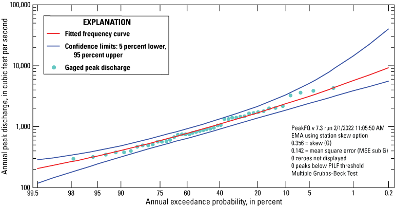
Example of output from flood-frequency software PeakFQ version 7.3 for U.S. Geological Survey station 16247000 Palolo Stream near Honolulu, Oʻahu, Hawaiʻi, using expected moments algorithm (EMA) with Multiple Grubbs-Beck Test and station skew only and data through water year 2020.
The mean describes the central tendency of the data. The standard deviation describes the spread or variability of the data. The skew describes the asymmetry of the distribution of data around the mean, as shown by the thicknesses of the tails of the distribution. For flood-frequency analysis, skew is generally the most uncertain variable because relatively short peak-flow records (less than 30 years) can lead to biased estimates of skew (Stedinger and others, 1993; England and others, 2019, p. 18). To help overcome the limitations with using short records to estimate skew, Bulletin 17C (England and others, 2019) recommends using a weighted skew computed from the streamgage-specific skew (at-site or station skew) and a generalized skew (regional skew) developed using data from many streamgages in a nearby area.
Regional Skew Coefficient
This section presents a general overview of the regional skew coefficient and criteria used for selection of sites in the regional skew analysis. More details about the regional skew regression analysis, including the methodology and calculations, are located in appendix 3.
To help improve estimates of annual peak discharges corresponding to various AEPs—particularly for streamgages with short annual peak-flow records (that is, streamgages with fewer than about 30 annual peaks)—current guidance for flood-frequency analysis by Federal agencies (Bulletin 17C; England and others, 2019) recommends using a weighted average of the at-site and regional skews. Previous guidance (Bulletin 17B; Interagency Advisory Committee on Water Data, 1982) supplied a national map of regional skew but encouraged hydrologists to develop more localized models when appropriate.
Because of complications introduced using EMA and MGBT (Cohn and others, 1997) and large cross-correlations between annual peak discharges at pairs of streamgages, a Bayesian weighted least-squares/Bayesian generalized least-squares (B–WLS/B–GLS) regression framework was developed to provide stable and defensible results for regional skew (Veilleux, 2011; Veilleux and others, 2011; Lamontagne and others, 2012; Veilleux and others, 2012). B–WLS/B–GLS uses ordinary least-squares (OLS) regression to fit an initial model of regional skew that is used to generate a stable estimate of regional skew for each streamgage. This estimate is the basis for computing the variance of each estimate of at-site skew used in the B–WLS analysis. B–WLS is then used to generate estimators of the regional skew model parameters. Finally, B–GLS is used to estimate the precision of those estimators, the model error variance and its precision, and compute various diagnostic statistics.
In this study, EMA with MGBT was used to estimate the at-site skew, G, and its mean squared error, MSEG. EMA with MGBT allows for the censoring of low floods as well as the use of flow intervals to describe missing, censored, and historical data. EMA with MGBT complicates the calculations of effective record length (and effective concurrent record length) used to describe the precision of skew estimates because the annual peak discharges are no longer represented by single values. To properly account for these complications, the B–WLS/B–GLS procedure was used.
A total of 124 streamgages that were not redundant (see section, “Elimination of Redundant Sites”) and had a pseudo effective record length (PRL) of 36 years or greater were used to develop the final regional skew model for Hawaiʻi (table 3.1, app. 3; for more information on pseudo effective record length, see app. 3). To explain the variability in skew, a windward/leeward split of flood regions and 17 basin characteristics were tested, but this approach failed to provide sufficient predictive power. Therefore, a constant regional skew (GR) of −0.157 was selected for the State of Hawaiʻi (app. 3). The average variance of prediction (AVPnew), 0.212, is equivalent to the mean square error of the regional skew (MSER) and corresponds to an effective record length of 36 years. These values supersede GR (−0.05), MSER (0.302), and effective record length of 17 years associated with the generalized skew map in Bulletin 17B (Interagency Advisory Committee on Water Data, 1982), which was used in the previous study (Oki and others, 2010).
Because of the relatively large uncertainty in the at-site skew for short to modest record lengths, the at-site skew and its MSE can be weighted with the regional skew and its MSE to generate a better, weighted estimate of skew for a given streamgage basin (Tasker, 1978; England and others, 2019, app. 7). Large deviations between the at-site and regional skew may indicate that the flood frequency characteristics of the basin of the streamgage of interest differ from those used to estimate the regional skew. If the at-site and regional skews differ by more than 0.5, it is considered reasonable to use the at-site skew instead of the weighted skew in the EMA (England and others, 2019, p. 25–26). The weighted skew was used within PeakFQ at all except the following streamgages, where the at-site skew was used: USGS streamgages 16400000 (Halawa Stream near Halawa, Molokaʻi), 16501200 (Oheo Gulch at dam near Kipahulu, Maui), 16502000 (Hahalawe Gulch near Kipahulu, Maui), 16557000 (Alo Stream near Huelo, Maui), 16565000 (Kaaiea Gulch near Huelo, Maui), 16638500 (Kahoma Stream at Lahaina, Maui), and 16717600 (Alia Stream near Hilo, Island of Hawaiʻi).
Expected Moments Algorithm Frequency Analysis
The guidelines in Bulletin 17C (England and others, 2019) suggest using the expected moments algorithm (EMA) to analyze the available flood data. EMA improves upon the methods provided in the previous flood-frequency guidelines, Bulletin 17B (Interagency Advisory Committee on Water Data, 1982), by cohesively incorporating all available flood-related data, including historical flood information, zero flows, low outliers, flow intervals, and perception thresholds (Lane and Cohn, 1996; Cohn and others, 1997; England and others, 2019).
Flood-frequency data generally come from two types of sources: systematic and historical data. Systematic data are the primary source of flood-frequency data for Hawaiʻi and consist of peak-flow data collected at regular intervals from either continuous-record gages or crest-stage gages. Systematic data are usually collected in consecutive years, although records sometimes contain data gaps between years (for example, see fig. 9). Historical data consist of major floods that exceeded a perception threshold and occurred outside the period of routine streamgaging, independent of how recently the flood occurred. Historical floods are valuable because they can be used to extend records with the knowledge that if a particular discharge was exceeded, it would have been recorded in some way. For example, at Kalihi Stream (USGS streamgage 16229300), historical data indicate that the flood on May 14, 1960, was the largest flood since at least 1937; with this information, the EMA can incorporate the period 1937–59 into the analysis by indicating that all annual peaks during this period were less than the peak discharge on May 14, 1960: 6,350 ft3/s.
Some peaks in the peak-flow record are classified as “opportunistic.” Opportunistic peaks occurred outside the period of systematic streamgaging and were measured because of operational decisions other than the exceedance of a perception threshold. Because the statistical sampling properties of opportunistic peaks are unknown, opportunistic peaks were excluded from flood-frequency analysis.
Flow Intervals and Perception Thresholds
Flow interval and perception thresholds must be defined in the PeakFQ program for every year with peak-flow data (table 4). The flow interval—represented by (QY,lower, QY,upper)—describes the annual-peak discharge which occurred. A flow interval can be (1) a discrete value, where a single peak is provided, or (2) a range, where the peak has some uncertainty (for example, less than, greater than, or between certain discharges). The perception threshold—represented by (TY,lower, TY,upper)—describes the range of discharges that would have been recorded had they occurred. The perceptible range is independent of the actual peak discharges that occurred. At streamgages with gaps in the systematic record, the perception threshold was set to (–100, infinity), and the flow interval was set to (0, infinity), which signifies to PeakFQ that the data are unavailable.
Table 4.
General perception-threshold and flow-interval settings applied to peak-flow data in the expected moments algorithm analysis to estimate peak-flow statistics at streamgages, State of Hawaiʻi.Continuous-Record Gages
At continuous-record gages, the peaks are usually discrete values known with confidence, and the flow intervals are represented as (QY, QY). In a few cases, where the peak discharge was estimated from historical information, a 20-percent uncertainty interval was applied to the estimated discharge. For example, an uncertain peak discharge listed as 100 ft3/s would be given a flow interval of (80, 120). Most continuous-record gages can record the full range of discharges; thus, the perception threshold for peaks from a continuous-record gage typically is (0, infinity).
Crest-Stage Gages
Crest-stage gages are simple devices designed to measure only the highest water stage over a given time period; flows below the bottom of the crest-stage gage—the gage base—are not recorded. The elevation of the gage base, which can change through time based on operational needs, is used to define the minimum recordable discharge (MRD) for a crest-stage gage at any given year. Consequently, crest-stage gages typically are given perception thresholds of (MRD, infinity). If the annual peak discharge did not exceed the MRD, the peak is recorded as a left-censored peak (“less than MRD”) and the flow interval is set as (0, MRD). If the annual peak discharge exceeded the MRD (uncensored peaks), the flow interval is set as (QY, QY). To estimate the MRDs for peaks determined from crest-stage gages, historical data were reviewed. If historical data were insufficient to estimate a MRD for a given year, the MRD was set to an estimated MRD from an adjacent record period; if a MRD could not be reasonably estimated for a crest-stage gage, the MRD was set to the lowest uncensored peak. Estimates of MRDs may be uncertain because (1) historical data sometimes lack the necessary information to estimate an MRD and (2) low flows at crest-stage gages are typically less important and the lower end of the stage-discharge relation is often poorly defined.
Low Outliers Identified with the Multiple Grubbs-Beck Test
Peak-flow records commonly contain low-magnitude outliers that deviate considerably from the rest of the peak population. Low outliers often have a disproportionately large influence on the fit of the frequency curve, at the expense of the fit at the high-discharge end of the curve (Cohn and others, 2013). Because most applications of flood-frequency analysis (for example, infrastructure design and flood protection) focus on the lower AEPs (larger peak flows), low outliers are removed when fitting the frequency curve. Bulletin 17C guidelines (England and others, 2019) recommend the Multiple Grubbs-Beck Test (MGBT) to detect and remove the potentially influential low floods (PILF) during flood-frequency analysis. The MGBT improves upon the Grubbs-Beck test (Grubbs and Beck, 1972) recommended in Bulletin 17B by accommodating the possibility that several low floods are potentially influential (Cohn and others, 2013; Lamontagne and others, 2016). The PeakFQ program, version 7.3, automatically applies the MGBT when computing flood statistics. For a few streamgages, a threshold for PILF detection and removal was manually set to improve the fit at the upper end of the frequency curve. For an example of a fitted frequency curve where PILFs have been removed, see figure 14.
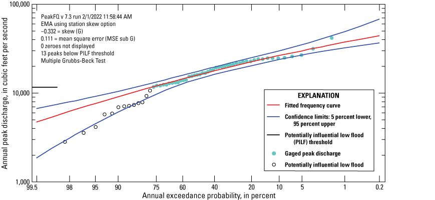
Example of output from flood-frequency software PeakFQ version 7.3 containing potentially influential low floods (PILF) for U.S. Geological Survey station 16103000 Hanalei River nr Hanalei, Kauaʻi, HI, using expected moments algorithm (EMA) with Multiple Grubbs-Beck Test and station skew only and data through water year 2020.
Flood-Frequency Estimates at Gaged Sites
Flood-frequency estimates for 238 streamgages in Hawaiʻi were calculated using EMA and MGBT techniques and the new regional skew coefficient (see section, “Regional Skew Coefficient”). The magnitude of peak flows for the 50-, 20-, 10-, 4-, 2-, 1-, 0.5-, and 0.2-percent AEPs are listed in appendix 4. Three estimates of peak flows for the select AEPs are provided: the at-site estimate (EMA), the regression-equation estimate (regression), and a weighted average of the other two estimates (weighted). The weighted estimate is generally preferred for most situations because it combines information from the independent at-station and regression-equation estimates (England and others, 2019, p. 33). The regression and weighted estimates will be discussed in subsequent sections.
Magnitude and Frequency of Floods at Ungaged Sites
Regression equations were developed to estimate peak-flow statistics at ungaged locations (the response variable) using basin characteristics (explanatory variables) determined for the ungaged location. The regression equations relate the AEP discharges determined from the EMA analysis to basin characteristics for streamgages in the study. The multiple-linear regression techniques used here follow the standard USGS methods outlined by Farmer and others (2019). Ordinary least-squares (OLS) regression was used in an exploratory data analysis to select the basin characteristics suitable for further evaluation. Generalized least-squares (GLS) regression was used to develop the final regression equations. The general form of the multiple-linear regression model is provided in the following equation:
whereYi
is the response variable (estimate of the streamflow magnitude) for site i;
b0 to bk
are the coefficients developed from the regression analysis;
X1 to Xk
are the k explanatory variables (basin characteristics); and
ei
is the residual error (difference between the observed and predicted values of the response variable) for site i.
The basic assumptions for multiple linear regression are (1) the model adequately describes the relation between the response variable and the explanatory variables, (2) variance of the residuals (ei) is constant (homoscedastic), (3) the residuals (ei) are independent of the explanatory variables (Xk), (4) the residuals (ei) are normally distributed, and (5) the residuals (ei) are independent of each other (Helsel and others, 2020, p. 228). The final assumption—residuals are independent of each other—is not satisfied by OLS regression because streamflow data generally are correlated in space and time, whereas GLS regression techniques account for spatial and temporal correlation. The OLS and GLS regression techniques are described in the following sections.
To improve the fit of the regression model, flood-frequency analyses commonly divide streamgages into spatial regions with similar hydrologic characteristics and develop independent models for each region. To evaluate possible regions for the current study, two statewide (based on data from Kauaʻi, Oʻahu, Molokaʻi, Maui, and the Island of Hawaiʻi) OLS regression equations were developed using drainage area as the only explanatory variable and the 0.10- and 0.01-AEP discharges as the response variables. The residuals for each streamgage—representing the difference between the peak discharge predicted from the OLS regression equations and the peak discharge obtained from the frequency curve for a streamgage using the EMA—were plotted on a map and the spatial patterns of residuals, along with topographic divides and hydrologic features, were evaluated to determine the final regional boundaries. Each of the five islands in the study area were split into two regions, resulting in 10 total regions (figs. 2–6). The regions used for Kauaʻi, Oʻahu, Molokaʻi, and the Island of Hawaiʻi match those used in the most recent USGS flood-frequency study for Hawaiʻi (Oki and others, 2010). For Maui, the regional boundary in the southeast was modified relative to Oki and others (2010) based on the spatial patterns of residuals in the OLS regression. The only streamgage in this study affected by the change in regional boundaries is USGS streamgage 16500100 (Kepuni Gulch near Kahikinui House, Maui), which switched from region 8 to 7.
Alternative regions were considered by testing combinations of streamgages on different islands with similar characteristics. For example, regions 5 (leeward Molokaʻi) and 7 (central-southwestern Maui) were combined and tested. Although the alternate regions did not result in improvements in performance metrics relative to the final regions used in this study, alternatives should be considered in future flood-frequency studies as a way to increase the sample size for areas with relatively few streamgages.
Elimination of Redundant Sites
Streamgages on the same stream and with similar size drainage basins may contain redundant hydrologic information. Redundant streamgages generally have similar basin characteristics and hydrologic responses to a given storm; thus, they provide only one unique statistical observation, rather than two independent observations. Including redundant streamgages in a regression analysis can negatively affect the results because the data are not independent (Farmer and others, 2019). To determine if two streamgages should be classified as redundant, three types of information are reviewed: (1) whether the streamgages have nested drainage basins, meaning that one drainage basin is entirely contained within the other, (2) whether the streamgages have drainage basins of similar size, and (3) whether the streamgages have temporal overlap in their peak-flow data.
To evaluate the likelihood that the streamgages have nested drainage basins, the standardized distance was computed. The standardized distance (SD) between two basin centroids is defined as:
whereDij
is the distance between centroids of basin i and basin j, in miles;
DAi
is the drainage area at streamgage i, in square miles; and
DAj
is the drainage area at streamgage j, in square miles.
A drainage area ratio was used to determine if the two streamgages had similarly sized drainage areas. The drainage area ratio (DAR) is defined as:
whereDAi
is the drainage area at site i, in square miles; and
DAj
is the drainage area at site j, in square miles.
A script written in the R programming language (R Core Team, 2021) was used to provide an initial screening of potentially redundant streamgages on the basis of the standardized distance and drainage area ratio. Screening thresholds for the standardized distance and drainage area ratio were set to 0.5 and 5, respectively. All possible combinations of streamgage pairs from the 238 streamgages were considered in the redundancy analysis. The script identified 50 potentially redundant pairs of streamgages (some streamgages were identified as potentially redundant to more than one other streamgage); 9 of the streamgage pairs identified were not nested or did not have temporal overlaps in their data and therefore were not considered redundant. For streamgage pairs that had nested basins and drainage area ratios less than five, one of the streamgages was classified as redundant and removed from the regression analysis. Generally, streamgages with longer periods of record were prioritized and retained. Additional considerations include (1) whether the streamgage is active and (2) how the streamgage’s basin characteristics fit into the distribution of basin characteristics for the streamgages in the region. For example, the streamgage with the largest drainage basin in the region may be prioritized, all other factors being equal, because it expands the range of values used to develop the regression equations (as will be discussed later, the regression equations should not be used with values for the explanatory variables that are not within the range of values used to develop the regression equations). Of the 238 streamgages considered for the regression analysis, 23 streamgages (about 10 percent) were classified as redundant and removed from the analysis (table 1.1, app. 1). Redundant streamgages were not included in either the regression or skew analyses, although station-specific flood statistics for redundant streamgages were still computed (table 1.1, app. 1).
Exploratory Data Analysis
An exploratory data analysis was completed to evaluate the best combinations of basin characteristics to use as explanatory variables in the regional regression equations. Scatter plots of each pair of response variable (flood discharge associated with an AEP) and explanatory variable (basin characteristic) were created to visually evaluate the pattern and linear relation between variables. Because multiple-linear regression seeks to quantify linear relations between the response and explanatory variables, data transformations were tested to improve the linearity of the relation. Logarithmic transformations (base 10) of both response and explanatory variables resulted in the best linear relations and the most constant variance (homoscedasticity) about the regression line. Prior to log transformation, a constant of 1 was added to the explanatory variables expressed as a percentage (for example, percentage impervious land cover) because some values for these basin characteristics are 0, and the logarithm of 0 is undefined. When logarithmic transformations are applied to the data to improve linearity, equation 2, which describes the general form of the regression model, becomes:
whereYi
is the response variable (estimate of the streamflow magnitude) for site i;
b0 to bk
are the coefficients developed from the regression analysis;
X1 to Xk
are the k explanatory variables (basin characteristics) for site i; and
ei
is the residual error (difference between the observed and predicted values of the response variable) for site i.
OLS regression analysis was performed using the R programming language (R Core Team, 2021) and the “smwrStats” statistical package (U.S. Geological Survey, 2017). An “all-possible subsets” regression was used to determine the best combinations of explanatory variables for models with 1–3 variables. Generally, the regression equations were limited to 1 variable per 10 streamgages in the region (Farmer and others, 2019). Model diagnostics for regression equations were reviewed for adequacy; selection criteria for explanatory variables included: (1) maximize the adjusted coefficient of determination, (2) minimize Mallow’s Cp statistic, and (3) minimize the predicted residual sum of squares (PRESS) statistic. Basin characteristics and the magnitude and sign of their coefficients in the regression equations were reviewed to ensure hydrologic plausibility. Multicollinearity, where two explanatory variables have a strong linear dependency, was evaluated using the variance inflation factor (VIF)—no variables in the final OLS regression models had a VIF greater than 5, indicating that multicollinearity is unlikely.
Regional Regression Equations
GLS multiple-linear regression (Stedinger and Tasker, 1985; Tasker and Stedinger, 1989; Farmer and others, 2019) was used to determine the final coefficients and performance metrics for each regional regression equation. GLS regression techniques are generally preferred for flood-frequency analysis because they improve estimates of AEP discharges and estimates of the accuracy of the regression model by accounting for (1) unequal record lengths from streamgages and (2) cross-correlation of streamflow statistics from streamgages (England and others, 2019, p. 30–31). Streamgages with shorter records are given less weight than streamgages with longer records. Additionally, less weight is given to streamgages where concurrent peak flows are correlated with nearby streamgages. Based on results from the OLS analysis, all explanatory and response variables were log-transformed prior to use in the GLS regression analysis. The USGS weighted-multiple-linear regression (WREG) program version 2.02 (https://github.com/USGS-R/WREG)—written in the R programming language (R Core Team, 2021)—was used to compute the final GLS equations and model performance metrics. Default values of the correlation-smoothing function in WREG (alpha, α, 0.002; and theta, θ, 0.98) were adjusted for each regional regression equation to improve model fit.
The final regression equations for estimating AEP discharges from basin characteristics for ungaged streams in Hawaiʻi are shown in table 5. Within each region, the explanatory variables were constrained to be identical for all regression equations; this ensures that predicted discharges uniformly increase as the AEP decreases. All explanatory variables used in the regression equations were statistically significant at the 95-percent confidence level (p-value less than or equal to 0.05) for at least one AEP in each region. Ranges of the explanatory variables used to develop the regression equations are presented in table 6.
Table 5.
Regional regression equations and performance metrics for estimating peak discharges for selected annual exceedance probabilities for ungaged streams in the State of Hawaiʻi.[Regression coefficients: Bold italics indicate that the associated explanatory variable was not statistically significant for the regression equation. Abbreviations: RMSE, root mean squared error; pseudo-R2, pseudo coefficient of determination; AVP, average variance of prediction; SEPavg, standard error of prediction; MEV, model error variance; SMEV, standard model error variance; WREG, weighted-multiple-linear regression program; --, not applicable; DRNAREA, drainage area (square miles); PRECIP, mean annual precipitation (inches); PERM24IN, area-weighted soil permeability for the top 24 inches of soil (inches per hour); I60M25Y, maximum 60-minute precipitation that occurs on average once in 25 years (inches); I48H500Y, maximum 48-hour precipitation that occurs on average once in 500 years (inches)]
Table 6.
Ranges of basin characteristics used to develop 10 regional regression equations, State of Hawaiʻi.[Abbreviations: --, not applicable; DRNAREA, drainage area (square miles); PRECIP, mean annual precipitation (inches); PERM24IN, area-weighted soil permeability for the top 24 inches of soil (inches per hour); I60M25Y, maximum 60-minute precipitation that occurs on average once in 25 years (inches); I48H500Y, maximum 48-hour precipitation that occurs on average once in 500 years (inches)]
Drainage area is the most common explanatory variable and appears in all equations except for those representing southern Island of Hawaiʻi (region 10). Other explanatory variables used in the regression equations include mean annual precipitation, precipitation-frequency statistics (for example, the maximum 48-hour rainfall that occurs on average once in 500 years, or I48H500Y), and soil permeability. The only region containing more than 1 explanatory variable per 10 streamgages was leeward Kauaʻi (region 1); here, a second explanatory variable—mean annual precipitation—was justified for the 17 streamgages in the region because of its clear hydrologic relation to flood magnitude and the notable improvement in performance metrics of the regression model, relative to a one-variable (drainage area) equation. All explanatory variables used in the regression equations except for soil permeability had positive coefficients, indicating that as the value of explanatory variable increases, the predicted flood discharge also increases.
Soil permeability was used as an explanatory variable in the leeward Oʻahu regression equations (region 3). The negative coefficient of the variable in all equations indicates that, as soil permeability increases, the predicted peak discharge decreases; this is intuitive because more permeable soils allow more water to infiltrate and reduce the volume of overland runoff than can contribute to flood peaks. The statistical significance of soil permeability decreases at the low-AEP floods and the p-value for soil permeability as a variable exceeds 0.05 at an AEP of 0.002. The importance of soil permeability is expected to be lower for the low-AEP floods because most soils become fully saturated during large flooding events; thus, the spatial variability of permeability will have a smaller influence on the flood magnitude above a certain threshold (Hollis, 1975; Konrad, 2003).
Southern Island of Hawaiʻi (region 10) is the only region where drainage area was not used as an explanatory variable. This may reflect the lack of well-defined stream channels in this area and the high permeabilities of soils and rocks at the surface (Oki and others, 2010). Because rainfall tends to infiltrate the surface quickly, drainage area likely does not play a large role in governing flood magnitudes for most AEPs in region 10.
Leverage and influence statistics computed by WREG were reviewed to evaluate how each streamgage affected the regression results. Leverage is a measure of how far away the values from one streamgage are from the values at all other streamgages in the regression model and is used to identify unusual observations (Farmer and others, 2019). Streamgages with high leverage have the potential to exert a strong influence on the regression parameters (Helsel and others, 2020, p. 238). The influence metric is a measure of how much influence a particular streamgage has on the regression parameters. Streamgages with leverage and influence values that exceeded the thresholds calculated by WREG were reviewed for potential errors in the peak-flow data (for example, poor computation of discharge from stage or inaccurate data representation in NWIS) and basin-characteristic data (for example, inaccurate basin delineations) or other issues that would make the streamgage ineligible for the regression model. Although several streamgages had both high leverage and influence, no errors were identified in the associated data and a reasonable hydrologic justification for removing the streamgages from the regression analysis could not be found.
Example Using a Peak-Flow Regression Equation
Example 1. Calculate the 0.01-AEP peak flow using the regional regression equations (Qreg) for USGS streamgage 16010000 on Kawaikoi Stream near Waimea, Kauaʻi, State of Hawaiʻi, at latitude 22°7’58.1” N and longitude 159°37’11.8” W. Streamgage 16010000 has a drainage area (DRNAREA) of 3.82 mi2 and a mean annual precipitation (PRECIP) of 133 inches.
Assessment of Fit
To assess the fit of the regression models, peak discharges predicted using the regression equations can be compared to the peak discharges determined from fitting the observed peak-flow data to the LP-III frequency curve (fig. 15). Comparisons of the observed and predicted peak discharges suggest that the regression models fit the observed data well. Additionally, plots of residuals (the difference between predicted and observed discharges) were examined to test the validity of the assumptions related to the regression models (fig. 16). The plots show that the residuals do not follow any trend and are equally distributed around zero and indicate that no model assumptions were violated.
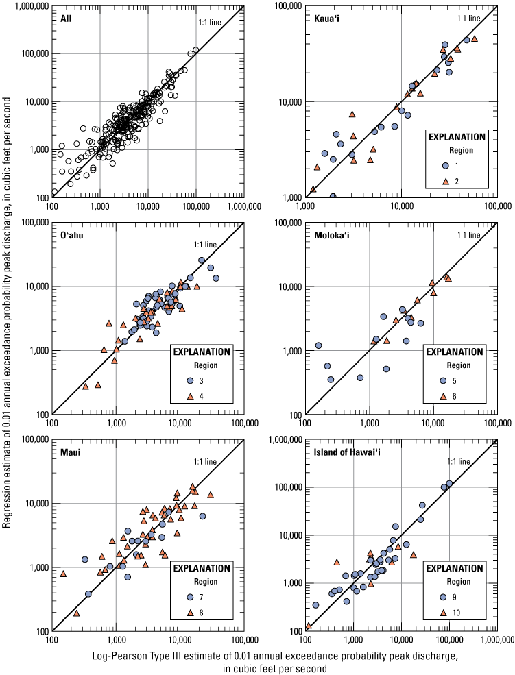
Comparisons between the 0.01 annual exceedance probability peak discharges estimated from the Log-Pearson Type III frequency curve and the regional regression equations, State of Hawaiʻi, using data through water year 2020.
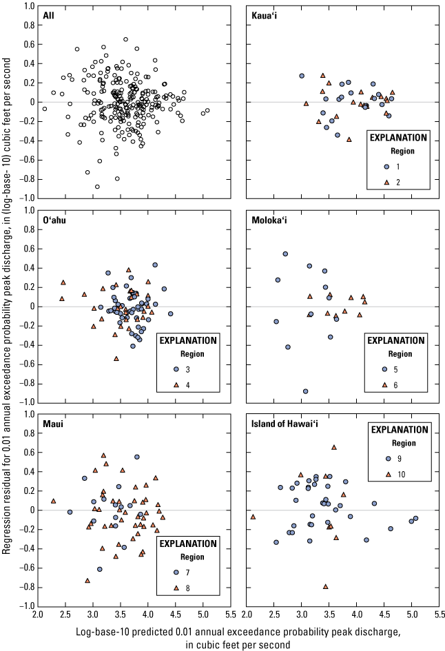
Residuals from the regional regression equations for the 0.01 annual exceedance probability peak discharges, State of Hawaiʻi, using data through water year 2020.
Accuracy and Limitations of Regional Regression Equations
Several performance metrics from the WREG program can be used to evaluate the accuracy of the regression equations. Performance metrics for the final regression equations are presented in table 5 and include the model error variance (MEV), the standard model error variance (SMEV), the root mean squared error (RMSE), the pseudo coefficient of determination (pseudo-R2), the average variance of prediction (AVP), and the average standard error of prediction (SEPavg). The MEV and SMEV describe the portion of the total error that can be attributed to having an imperfect model, in log units and percent, respectively. The RMSE and pseudo-R2 are measures of model accuracy for streamgages used in the model development. RMSE describes how much the predicted peak discharges deviate from the observed peak discharges. The pseudo-R2 is a measure of the predictive strength of the regression model and describes the variability of the response variable that is explained by the explanatory variables, after accounting for the effect of time-sampling error. The pseudo-R2 is similar to the standard coefficient of determination (R2), where the closer the value is to 1.0 (or 100 percent), the greater the amount of variance that is explained by the regression. The AVP and SEPavg are measures of how well the regression model performs at predicting peak discharges for ungaged sites not used to develop the regression equations—lower values indicate greater predictive power. Generally, pseudo-R2 and AVP were the most important metrics for selecting the final regression equations. Equations for calculating these performance metrics are available in Eng and others (2009).
The pseudo-R2 values for the final regression equations ranged from 11.9 percent (region 7; 0.5 AEP) to 100.0 percent (region 6; 0.002–0.02 AEPs) for all regions and AEPs, and ranged from 46.2 percent (region 5) to 100.0 percent (region 6) for the 0.01-AEP discharges. The AVP values for the final regression equations ranged from 0.0046 (region 6; 0.02 AEP) to 0.3400 (region 5; 0.5 AEP) for all regions and AEPs, and ranged from 0.0062 (region 6) to 0.2455 (region 10) for the 0.01-AEP discharges. Overall, the final regression models performed well for all regions except regions 5 and 10. The large errors associated with the regression equations for regions 5 (leeward Molokaʻi) and 10 (southern Island of Hawaiʻi) reflect the relatively few sites and short records available and the poor understanding of flood-producing mechanisms in these areas. Collection of additional peak-flow data and consideration of basin characteristics that better characterize flood conditions may improve the accuracy of regression equations used to predict peak flows at ungaged sites in these regions.
The accuracy of the regression equations may be affected by issues associated with the explanatory and response variables. The basin characteristics used as explanatory variables rely on accurate basin delineations—any change to the basin delineations will affect the computed values for each basin characteristic, even if the source data for the basin characteristics remain unchanged. Future analyses that use higher-resolution DEMs (for example, DEMs derived from light detection and ranging [lidar] data) to delineate basins will result in improved accuracy for basin characteristics used in the regression analyses. Potential errors associated with the peak-flow statistics used as response variables in the regression equations include non-representative data from streamgages with short records and errors computing discharge from stream stage (Turnipseed and Sauer, 2010).
The explanatory variables (basin characteristics) should be representative of basin conditions during the period of record that was used to derive the response variables (peak-flow statistics) (Farmer and others, 2019). The historical periods used to determine the mean annual precipitation, precipitation-frequency statistics, and soil permeability used in the final regression equations were 1978–2007, 1899–2005, and 2001–19, respectively. The peak-flow statistics used as response variables were determined from peak-flow data collected during 1911–2021; however, the temporal availability of peak-flow data for each region varies substantially (for example, see fig. 9). If a streamgage used in the regression analysis only has peak-flow data collected during a particularly wet period (for example, the 1960s), it may not accurately characterize the expected long-term relation between basin characteristics and peak-flow statistics in the region.
The regression equations are only applicable to ungaged locations with basin characteristics within the range of values used to develop the regression equations (table 6). If the regression equations are used beyond these limits, the accuracy of the estimated peak-flow statistics would be unknown. Additionally, basin characteristics at ungaged sites should be computed using the same datasets and methods as were used in this study. The USGS StreamStats web application provides the same datasets and methods as were used in this study and therefore provides the most consistent way to estimate peak-flow statistics at ungaged sites (see section, “Estimating Flow Statistics Using StreamStats”). The regression equations developed in this study apply to stream sites that are unregulated and have less than 20 percent impervious land cover; however, StreamStats is unable to warn users or prevent them from selecting regulated stream sites because identifying all stream sites in the study area that are substantially affected by regulations is challenging.
Uncertainty of Individual Estimates Computed Using the Regression Equations
When applying the regression equations at ungaged sites not used in the development of the regression equations, it is important to understand the accuracy and uncertainty associated with the estimated discharge. Two commonly used metrics for the accuracy of an estimated discharge at a particular site are the variance of prediction (VP) and the standard error of prediction (SEP). For a site i, the variance of prediction is the sum of the model error variance and the sampling error variance. The variance of prediction for each streamgage used in the development of the regression equations is computed in WREG. To compute the variance of prediction for estimated discharges using the regression equations (), the following equation can be applied:
whereis the variance of prediction for site i, in log units;
is the model error variance (see table 5 for values), in log units; and
is the sampling error variance for site i, in log units.
The sampling error variance is computed as follows:
whereis a row vector of the regressor (basin characteristic) variables associated with site i, augmented by a value of 1.0 in the first column;
is the (1 × p) matrix consisting of 1 row and the p-1 regressor variables augmented by a column of ones in the first column;
is the (n by n) covariance matrix used for weighting sample data in the GLS regression;
is the covariance matrix for the regression coefficients (Mitchell and Wagner, 2022);
and
are the superscripts indicating the transpose and inverse of the matrices, respectively;
is the number of streamgages used in the regression analysis; and
is the number of basin characteristics in the regression equation plus 1.
The SEP for site i, expressed in log units, can be computed as:
whereTo understand the uncertainty of an individual discharge estimate when using the regression equations at an ungaged site, prediction intervals can be computed. Prediction intervals combine the uncertainty of the regression parameters and placement of the regression line—typically described by confidence intervals—with the uncertainty associated with the residuals (Farmer and others, 2019). Prediction intervals describe the range of values within a specific confidence interval, within which the true value exists (Helsel and others, 2020). The following equations can be used to compute the 95-percent prediction intervals for peak-flow estimates obtained using the regression equations for ungaged locations:
where,
are the upper and lower prediction intervals, respectively, for a given AEP at site i;
is the predicted discharge for a given AEP at site i, in log units;
is Student’s t with a specified alpha (α) level and n−p degrees of freedom, where n is the number of sites used in the regression equation and p is the number of regressor variables plus 1 (values for each regression region are listed in table 5); and
is the variance of prediction for a given AEP at site i, in log units, computed using equations 6 and 7.
For sites not used in the development of the regression equations, the average variance of prediction (AVP), available in table 5, should be substituted for the site-specific variance of prediction () in equations 9 and 10.
Application of Methods
The techniques for estimating peak discharges described in this report can be applied to three different situations:
-
1. A gaged location with at least 10 usable annual peaks.
-
2. An ungaged location or a gaged location with less than 10 usable annual peaks located near a streamgage for which peak-flow statistics have been or can be computed.
-
3. An ungaged location or a gaged location with less than 10 usable annual peaks not located near a streamgage for which peak-flow statistics have been or can be computed.
The methods for the first two situations are described below. For the third situation, the appropriate regression equation in table 5 should be applied directly to estimate peak discharges (see section, “Estimating Flow Statistics Using StreamStats”).
Weighting Flood-Frequency Estimates at Gaged Sites
An improved estimate of peak discharge can be obtained for gaged sites by combining information from the at-site flood-frequency curve (that is, EMA) with information from the regional regression equations (England and others, 2019). The two estimates of peak discharge can be considered independent if the regression equations were developed with a large number of sites. The combined peak-flow estimate is weighted based on the inverse of the variance of prediction for each independent estimate. The weighting procedure only applies to unregulated streams with minimal basin urbanization. The weighted discharges are available in appendix 4 (and can be accessed using StreamStats) and were computed with the following equation:
whereis the weighted-discharge estimate for a given AEP at site i, in cubic feet per second;
is the variance of prediction at the streamgage for a given AEP at site i, in log units, derived from the applicable regional regression equation;
is the EMA-discharge estimate for a given AEP at site i, in cubic feet per second;
is the variance of prediction at the streamgage for a given AEP at site i, in log units, derived from the EMA analysis; and
is the regression-discharge estimate for a given AEP at site i, in cubic feet per second.
The variance of prediction for the weighted-discharge estimate () can be computed as follows:
Once and have been determined, the upper and lower prediction intervals for the weighted-discharge estimate can be computed as follows:
where,
are the upper and lower prediction intervals, respectively, for a given AEP at site i;
is the weighted-discharge estimate for a given AEP at site i;
is Student’s t with a specified alpha (α) level and n−p degrees of freedom, where n is the number of sites used in the regression equation and p is the number of regressor variables plus 1 (values are listed in table 5); and
is the variance of prediction of the weighted-discharge estimate for a given AEP at site i, in log units.
Example of Weighting a Peak-Flow Estimate with Observed and Predicted Values
Example 2. Calculate the 0.01-AEP (or 1.0-percent AEP) weighted peak flow (Qwtd) for USGS streamgage 16010000 on Kawaikoi Stream near Waimea, Kauaʻi, State of Hawaiʻi, at latitude 22°7’58.1” N and longitude 159°37’11.8” W. Streamgage 16010000 has a drainage area (DRNAREA) of 3.82 mi2 and a mean annual precipitation (PRECIP) of 133 inches.
-
1. From example 1 and appendix 4, a predicted 0.01-AEP peak-flow estimate (Qreg) of 7,240 ft3/s (converted to 3.860 ft3/s log units) was computed using the appropriate regression equation for region 1 (table 5).
-
2. From appendix 4, the variance of prediction for the regression estimate (VPreg) is reported as 0.0230 log units.
-
3. From appendix 4, the observed 0.01-AEP peak-flow estimate (QEMA) and corresponding at-site variance of prediction (VPreg) are reported as 11,600 ft3/s (converted to 4.064 ft3/s log units) and 0.0031 log units, respectively.
-
4. Using equation 11, a weighted peak-flow estimate (Qwtd) can be computed as follows:
Weighting Flood-Frequency Estimates at Ungaged Sites with Data from a Nearby Gage
Peak-flow estimates determined using the regional regression equations for ungaged sites can be improved if the ungaged site is located near a gaged site on the same unregulated stream. This approach combines information from the regression equations at the ungaged site with information from the discharge estimates at a nearby gaged site by, in part, relating the drainage areas of the two sites. The weight of the regression-derived discharge estimate for the ungaged site increases relative to the weight of the discharge estimates from the gaged site as the drainage-area ratio increases (that is, as the distance between the two sites increases). To apply this weighting method, the gaged site must have at least 10 years of peak-flow data, and the ungaged site must have a drainage area within 50 percent of the drainage area of the gaged site (the drainage-area ratio is more than 0.5 and less than 1.5) and must be located on the same stream (Ries, 2007; Feaster and others, 2009). The following equation can be used to compute the weighted-discharge estimate at the ungaged site:
whereis the weighted-discharge estimate at the ungaged site for a given AEP, in cubic feet per second;
is absolute value of the difference between the drainage areas of the gaged and ungaged sites, in square miles;
is the drainage area for the gaged site, in square miles;
is the weighted-discharge estimate at the gaged site for a given AEP, in cubic feet per second;
is the discharge estimate computed using the applicable regional regression equation at the gaged site for a given AEP, in cubic feet per second; and
is the discharge estimate computed using the applicable regional regression equation at the ungaged site for a given AEP, in cubic feet per second.
Comparison of Results with Previous Studies
The weighted peak-flow estimates and regression equations were compared to the results from the most recent USGS flood-frequency analysis in Hawaiʻi (Oki and others, 2010). For most of the 220 streamgages included in both this study and Oki and others (2010), the weighted peak-flow estimates for the 0.01 AEP were similar (fig. 17). The median relative difference for weighted peak-flow estimates in each region ranged from −4 to 0 percent, indicating a slight decrease in peak-flow estimates. Generally, larger relative differences in the estimated peak flows are observed for the smaller AEPs (largest floods) than for the larger AEPs (smallest floods) (fig. 18).
The regional regression equations in this study provide more accurate estimates for some regions and similarly accurate estimates in other regions, compared to the equations developed by Oki and others (2010). Performance metrics for the regression equations indicate improvements in regions 1, 3, 4, 7, 8, and 10, and similar metrics in regions 2, 5, 6, and 9 (table 7). Improvements in model performance for regions 1, 3, 4, and 8 can be partly attributed to the addition of a new variable that was not used in Oki and others (2010).
Differences in the weighted peak-flow estimates and regression performance metrics in this study relative to Oki and others (2010) may be explained by several factors, including variable selection for the regression equations, data availability, streamgage selection, regional skew, and flood-frequency techniques. This study used data through water year 2020, whereas Oki and others (2010) used data through water year 2008; the additional 12 years of peak-flow data have greater potential to influence estimated flood statistics at streamgages with short records compared to those with long records. In addition to data availability, the criteria used to select streamgages—including the removal of redundant streamgages from the development of the regression equations—differed between the two studies. The regional skew for this study (−0.157 and a MSE of 0.212) was developed following updated national guidelines (Bulletin 17C; England and others, 2019) and B–WLS/B–GLS methods; the regional skew used by Oki and others (2010) (−0.05 and a MSE of 0.302) was computed as the arithmetic mean of at-site skews from 30 streamgages with data through water year 1973 (Bulletin 17B; Interagency Advisory Committee on Water Data, 1982). Lastly, the use of EMA with MGBT for this study likely improved at-site estimates of peak discharge for streamgages with censored, interval, or historical data types, relative to the at-site estimates from Oki and others (2010), which were computed using techniques described in Bulletin 17B.
Table 7.
Selected results of regional peak-flow regression equations developed by this study compared to those from Oki and others (2010).[Abbreviations: SEP, standard error of prediction; AEP, annual exceedance probability; SME, standard model error; DRNAREA, drainage area (square miles); PRECIP, mean annual precipitation (inches); PERM24IN, area-weighted soil permeability for the top 24 inches of soil (inches per hour); I60M25Y, maximum 60-minute precipitation that occurs on average once in 25 years (inches); I48H500Y, maximum 48-hour precipitation that occurs on average once in 500 years (inches); I48H5Y, maximum 48-hour precipitation that occurs on average once in 5 years (inches); I48H2Y, maximum 48-hour precipitation that occurs on average once in 2 years (inches); pseudo-R2, pseudo coefficient of determination; AVP, average variance of prediction]
| Region | Number of sites used | Variables used | Average SEP at all shared AEPs, in percent | SEP at the 0.01 AEP, in percent | Average SME at all shared AEPs, in percent | SME at the 0.01 AEP, in percent | Average pseudo-R2 at all shared AEPs, in percent | Pseudo-R2 at the 0.01 AEP, in percent | ||||||||
|---|---|---|---|---|---|---|---|---|---|---|---|---|---|---|---|---|
| This study | Oki and others (2010) | This study | Oki and others (2010) | This study | Oki and others (2010) | This study | Oki and others (2010) | This study | Oki and others (2010) | This study | Oki and others (2010) | This study | Oki and others (2010) | This study | Oki and others (2010) | |
| 1 | 17 | 19 | DRNAREA; PRECIP | DRNAREA | 42 | 63 | 39 | 53 | 37 | 59 | 34 | 49 | 90 | 76 | 91 | 82 |
| 2 | 16 | 18 | DRNAREA | DRNAREA | 47 | 44 | 33 | 32 | 43 | 40 | 29 | 28 | 90 | 91 | 94 | 94 |
| 3 | 43 | 47 | DRNAREA; PRECIP; PERM24IN | DRNAREA; PRECIP | 35 | 43 | 31 | 41 | 32 | 40 | 28 | 38 | 84 | 75 | 83 | 75 |
| 4 | 26 | 24 | DRNAREA; I60M25Y | DRNAREA | 39 | 51 | 37 | 48 | 35 | 47 | 33 | 44 | 90 | 83 | 90 | 84 |
| 5 | 12 | 11 | DRNAREA | DRNAREA | 153 | 199 | 129 | 110 | 133 | 161 | 113 | 96 | 41 | 38 | 46 | 51 |
| 6 | 9 | 10 | DRNAREA | DRNAREA | 23 | 21 | 18 | 17 | 11 | 14 | 0 | 6 | 98 | 97 | 100 | 99 |
| 17 | 15 | 14 | DRNAREA | DRNAREA | 70 | 107 | 50 | 67 | 61 | 90 | 43 | 54 | 69 | 62 | 82 | 76 |
| 18 | 40 | 44 | DRNAREA; PRECIP | DRNAREA | 58 | 73 | 68 | 70 | 55 | 70 | 64 | 67 | 81 | 69 | 75 | 69 |
| 9 | 30 | 34 | DRNAREA; PRECIP | DRNAREA; PRECIP | 57 | 63 | 47 | 51 | 51 | 57 | 42 | 44 | 86 | 87 | 90 | 91 |
| 10 | 9 | 11 | I48H500Y | I48H5Y2 | 152 | 159 | 164 | 170 | 128 | 136 | 136 | 140 | 51 | 32 | 53 | 37 |
Station 16500100, which changed from region 8 in Oki and others (2010) to region 7 in this study, is included in the respective regions and performance metrics.
I48H2Y was used at the 0.5 AEP in Oki and others (2010).
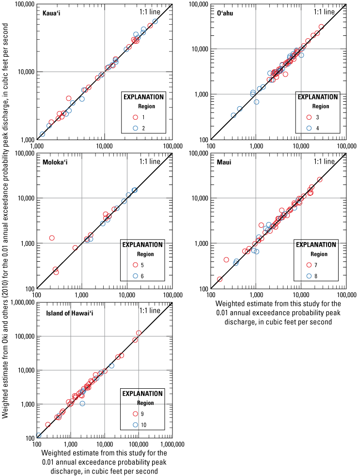
Comparisons between the 0.01 annual exceedance probability peak discharges from this study—using data through water year 2020—with the previously published estimates from Oki and others (2010) for the 220 streamgages included in both studies.
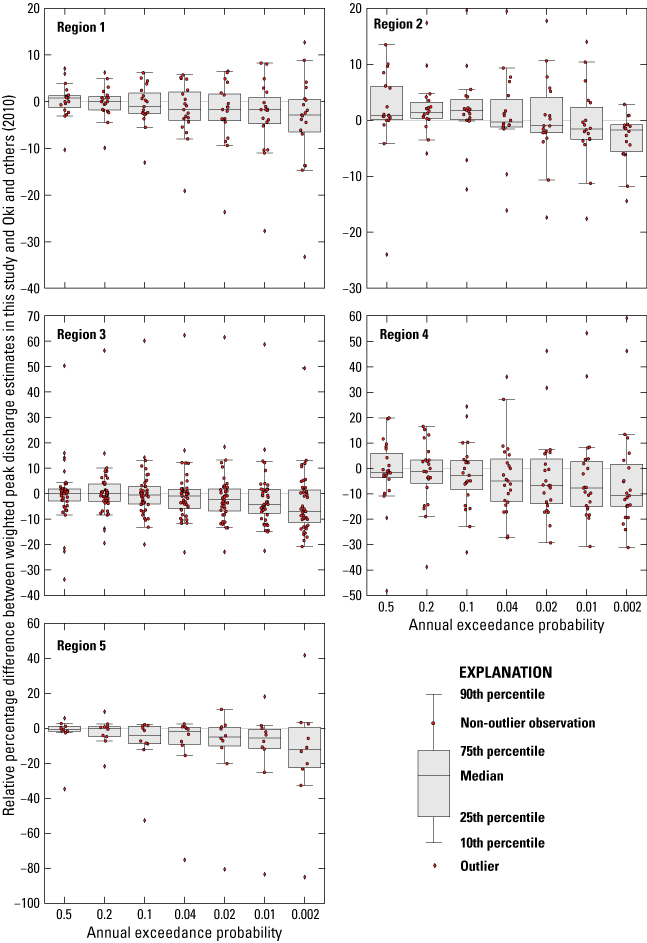
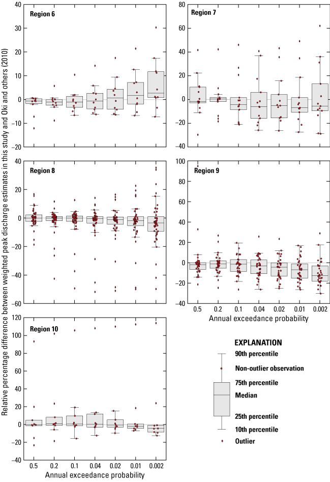
Comparisons between the annual exceedance probability (AEP) peak discharges from this study—using data through water year 2020—and the previously published estimates from Oki and others (2010) for the 220 streamgages included in both studies. The 0.005 AEP was not used in Oki and others (2010) and is not included here. The relative percentage differences for streamgage number 164118000 in region 5 are not shown because they would limit the ability to view the other data in this region; at an AEP of 0.5, this study estimated a weighted discharge of 26 cubic feet per second, and Oki and others (2010) estimated a weighted discharge of 3.5 cubic feet per second, resulting in a relative difference of 643 percent.
Estimating Flow Statistics Using StreamStats
The USGS StreamStats program (U.S. Geological Survey, 2019, https://streamstats.usgs.gov) is a web-based GIS application that provides users with several analytical tools for water-resources planning and management (Rosa and Oki, 2010; Ries and others, 2017). One of the core capabilities of StreamStats is that it allows users to select an ungaged location on a stream network to delineate a drainage basin, compute basin characteristics, and calculate selected streamflow statistics (for example, peak-flow, low-flow, and flow-duration statistics). StreamStats provides a faster, more accurate, and more consistent approach for estimating streamflow statistics at ungaged locations than manual methods.
The basin characteristics (table 3) and regional regression equations (table 5) described in this study have been integrated into the USGS StreamStats program for Hawaiʻi. If users select an ungaged location in StreamStats, they will be able to delineate a drainage basin, compute selected basin characteristics, and estimate selected flow statistics—including the AEP discharges reported in this study. If the ungaged location selected by the user has basin characteristics within the range of those used to develop the applicable regression equations, StreamStats will provide available accuracy metrics and prediction intervals for the peak-flow estimates (described in section, “Accuracy and Limitations of Regional Regression Equations”). StreamStats currently does not have the ability to weight the peak-flow estimate at an ungaged location with the peak-flow estimates from a nearby gaged location (described in section, “Weighting Flood-Frequency Estimates at Ungaged Sites with Data from a Nearby Gage”)—these computations will need to be completed manually using the regression-derived discharge estimate at the ungaged site and the discharge estimates provided by StreamStats for the nearby gaged site. If a user selects a gaged location in StreamStats, they can obtain the full suite of available basin characteristics and flow statistics, including those not reported in this study (for example, low-flow statistics, if available). Additionally, published basin characteristics and flow statistics at streamgages can be accessed on StreamStats directly at https://streamstatsags.cr.usgs.gov/gagepages/html/00000000.htm (U.S. Geological Survey, 2019), where 00000000 is substituted with the station number for the streamgage.
Summary
The U.S. Geological Survey (USGS), in cooperation with the State of Hawaiʻi Department of Transportation, updated flood estimates for the 50-, 20-, 10-, 4-, 2-, 1-, 0.5-, and 0.2-percent annual exceedance probabilities (AEP) for unregulated streamgages in Kauaʻi, Oʻahu, Molokaʻi, Maui, and Hawaiʻi, State of Hawaiʻi. Regression equations which can be used to estimate flood magnitude and associated frequency at ungaged streams were developed. This study uses data through water year 2020 and supersedes the previous USGS flood-frequency report, Oki and others (2010), which used data through water year 2008.
Flood magnitude and frequency at 238 streamgages were estimated—following national guidelines established in Bulletin 17C (England and others, 2019)—by fitting annual peak-flow data to the Log-Pearson Type III distribution using the expected moments algorithm (EMA) and the USGS PeakFQ flood-frequency software. Potentially influential low outliers in the data were identified and removed using the Multiple Grubbs-Beck Test. An updated regional skewness coefficient (regional skew) for Hawaiʻi was estimated using the Bayesian weighted least squares/Bayesian generalized least squares (B–WLS/B–GLS) method. The B–WLS/B–GLS method for determining regional skew accounts for complexities introduced by EMA and the cross-correlation of annual peak flows at pairs of streamgages, resulting in a more accurate estimate of regional skew and a better understanding of uncertainty. The updated regional skew employs a constant model for the five islands in the study area and has a value of −0.157 (mean square error of 0.212).
Trends in the peak-flow data were evaluated to test the statistical assumptions for flood-frequency analysis described in Bulletin 17C. Monotonic trends, representing a unidirectional change over time, were evaluated using three versions of the nonparametric Mann-Kendall test. Step trends, representing abrupt shifts in the statistical properties of time-series data, were evaluated using the Pettitt test. About 21 percent of streamgages had a significant monotonic trend with at least one version of the Mann-Kendall test; streamgages on Kauaʻi, Oʻahu, and the Island of Hawaiʻi had predominantly decreasing trends, whereas streamgages on Maui and Molokaʻi had mixed results. About 18 percent of streamgages had a significant step trend; 26 streamgages with significant step trends had peak-flow magnitudes that decreased after the change point and 18 streamgages had peak-flow magnitudes that increased after the change point. Although this study only represents a cursory trend analysis, the observed trends do not have clear deterministic relations with known hydroclimatological or land-use changes. Consequently, no streamgages were removed from the analysis and the statistical assumptions were presumed to be valid. Trends should continue to be evaluated in future flood-frequency analyses, particularly if techniques capable of adjusting data for definitive nonstationarities become readily available.
Multiple-linear regression techniques were used to relate basin characteristics to peak flows at streamgages for the purposes of estimating peak flows at ungaged sites. The study area was split into 10 regions—two regions per island, generally following a leeward/windward split—containing from 9 to 49 streamgages each. Fifty-eight basin characteristics, representing physical or climatic attributes that may relate to flood statistics, were computed for each streamgage. Ordinary least squares regression methods were used in an exploratory data analysis to select candidate explanatory variables (basin characteristics). The final regression equations for each region were determined with generalized least squares methods using the USGS weighted-multiple-linear regression (WREG) program. The standard error of prediction at the 0.01 AEP for the regression equations ranged from 18 to 164 percent; the pseudo coefficient of determination (pseudo-R2) at the 1-percent AEP ranged from 46 to 100 percent. The regression equations performed well for all regions except leeward Molokaʻi and southern Island of Hawaiʻi; for all other regions, the pseudo-R2 ranged from about 75 to 100 percent. Compared to the regression equations developed by Oki and others (2010), the regression equations in this study generally had greater accuracy and predictive power, although the degree of improvement varied for each region. The regression equations are only applicable to locations with basin characteristics within the range of values used to develop the regression equations.
At streamgages with data analyzed in this study, final peak-flow estimates are weighted using the at-site statistics computed with PeakFQ and the predicted flows from the regression equations. Results of this study—including the final peak-flow estimates at streamgages and the regression equations—are implemented in the USGS StreamStats web application (U.S. Geological Survey, 2019). StreamStats provides the most consistent approach for obtaining peak-flow estimates at streamgages and for applying the regional regression equations for estimating peak flows at ungaged locations.
References Cited
Barnhart, T.B., Smith, M., Rea, A., Kolb, K., Steeves, P., and McCarthy, P., 2020, StreamStats data preparation tools, version 4: U.S. Geological Survey software release, accessed October 5, 2022, at https://doi.org/10.5066/P9UM2NUL.
Cao, G., Giambelluca, T.W., Stevens, D.E., and Schroeder, T.A., 2007, Inversion variability in the Hawaiian trade wind regime: American Meteorological Society, v. 20, no. 7, p. 1145–1160, accessed May 17, 2021, at https://doi.org/10.1175/JCLI4033.1.
Caruso, S.J., and Businger, S., 2006, Subtropical cyclogenesis over the central North Pacific: Weather and Forecasting, v. 21, no. 2, p. 193–205, accessed June 3, 2021, at https://doi.org/10.1175/WAF914.1.
Chen, Y.R., and Chu, P.-S., 2014, Trends in precipitation extremes and return levels in the Hawaiian Islands under a changing climate: International Journal of Climatology, v. 34, no. 15, p. 3913–3925, accessed April 6, 2021, at https://doi.org/10.1002/joc.3950.
Chen, Y.-L., and Feng, J., 1995, The influences of inversion height on precipitation and airflow over the Island of Hawaii: Monthly Weather Review, v. 123, no. 6, p. 1660–1676, accessed June 4, 2021, at https://doi.org/10.1175/1520-0493(1995)123%3C1660:TIOIHO%3E2.0.CO;2.
Chu, P.-S., 1995, Hawaii rainfall anomalies and El Niño: American Meteorological Society, v. 8, no. 6, p. 1697–1673, accessed June 3, 2021, at https://doi.org/10.1175/1520-0442(1995)008%3C1697:HRAAEN%3E2.0.CO;2.
Chu, P.-S., and Chen, H., 2005, Interannual and interdecadal rainfall variations in the Hawaiian Islands: Journal of Climate, v. 18, no. 22, p. 4796–4813, accessed April 29, 2021, at https://doi.org/10.1175/JCLI3578.1.
Chu, P.-S., Chen, Y.R., and Schroeder, T.A., 2010, Changes in precipitation extremes in the Hawaiian Islands in a warming climate: American Meteorological Society, v. 23, no. 18, p. 4881–4900, accessed April 6, 2021, at https://doi.org/10.1175/2010JCLI3484.1.
Chu, P.-S., Nash, A.J., and Porter, F.-Y., 1993, Diagnostic studies of two contrasting rainfall episodes in Hawaii—Dry 1981 and wet 1982: American Meteorological Society, v. 6, no. 7, p. 1457–1462, accessed May 18, 2021, at https://doi.org/10.1175/1520-0442(1993)006%3C1457:DSOTCR%3E2.0.CO;2.
Cohn, T.A., England, J.F., Berenbrock, C.E., Mason, R.R., Stedinger, J.R., and Lamontagne, J.R., 2013, A generalized Grubbs-Beck test statistic for detecting multiple potentially influential low outliers in flood series: Water Resources Research, v. 49, no. 8, p. 5047–5058, accessed March 5, 2020, at https://doi.org/10.1002/wrcr.20392.
Cohn, T.A., Lane, W.L., and Baier, W.G., 1997, An algorithm for computing moments-based flood quantile estimates when historical flood information is available: Water Resources Research, v. 33, p. 2089–2096, accessed March 5, 2020, at https://doi.org/10.1029/97WR01640.
Cohn, T.A., and Lins, H.F., 2005, Nature’s style—Naturally trendy: Geophysical Research Letters, v. 32, no, 23, 5 p, accessed May 5, 2020, at https://doi.org/10.1029/2005GL024476.
Diaz, H.F., and Giambelluca, T.W., 2012, Changes in atmospheric circulation patterns associated with high and low rainfall regimes in the Hawaiian Islands region on multiple time scales: Global and Planetary Change, v. 98–99, p. 97–108, accessed June 4, 2021, at https://doi.org/10.1016/j.gloplacha.2012.08.011.
Dudley, R.W., Archfield, S.A., Hodgkins, G.A., Renard, B., and Ryberg, K.R., 2018, Peak-streamflow trends and change-points and basin characteristics for 2,683 U.S. Geological Survey streamgages in the conterminous U.S. (ver. 3.0, April 2019): U.S. Geological Survey data release, accessed June 4, 2021, at https://doi.org/10.5066/P9AEGXY0.
Dudley, R., Hodgkins, G., Mann, A., and Chisholm, J., 2001, Evaluation of the effects of development on peak-flow hydrographs for Collyer Brook, Maine: U.S. Geological Survey Water-Resources Investigations Report 01–4156, 11 p., accessed June 9, 2021, at https://doi.org/10.3133/wri20014156.
Elison Timm, O., Diaz, H.F., Giambelluca, T.W., and Takahashi, M., 2011, Projection of changes in the frequency of heavy rain events over Hawaii based on leading Pacific climate modes: Journal of Geophysical Research, v. 116, no. D4, 12 p., accessed May 5, 2021, at https://doi.org/10.1029/2010JD014923.
Elison Timm, O., Li, S., Liu, J., and Beilman, D.W., 2020, On the changing relationship between North Pacific climate variability and synoptic activity over the Hawaiian Islands: International Journal of Climatology, v. 41, no. S1, p. E1566–E1582, accessed May 5, 2021, at https://doi.org/10.1002/joc.6789.
Eng, K., Chen, Y.-Y., and Kiang, J.E., 2009, User’s guide to the weighted-multiple-linear regression program (WREG version 1.0): U.S. Geological Survey Techniques and Methods, book 4, chap. A8, 21 p., accessed April 1, 2020, at https://doi.org/10.3133/tm4A8.
England, J.F., Jr., Cohn, T.A., Faber, B.A., Stedinger, J.R., Thomas, W.O., Jr., Veilleux, A.G., Kiang, J.E., and Mason, R.R., Jr., 2019, Guidelines for determining flood flow frequency—Bulletin 17C (ver. 1.1, May 2019): U.S. Geological Survey Techniques and Methods, book 4, chap. B5, 148 p., accessed April 1, 2020, at https://doi.org/10.3133/tm4B5.
Farmer, W.H., Kiang, J.E., Feaster, T.D., and Eng, K., 2019, Regionalization of surface-water statistics using multiple linear regression (ver. 1.1, February 2021): U.S. Geological Survey Techniques and Methods, book 4, chap. A12, 40 p., accessed May 3, 2021, at https://doi.org/10.3133/tm4A12.
Feaster, T.D., Gotvald, A.J., and Weaver, J.C., 2009, Magnitude and frequency of rural floods in the Southeastern United States, 2006; Volume 3, South Carolina: U.S. Geological Survey Scientific Investigations Report 2009–5156, 226 p., accessed February 23, 2022, at https://doi.org/10.3133/sir20095156.
Flynn, K.M., Kirby, W.H., and Hummel, P.R., 2006, User’s manual for program PeakFQ, annual flood-frequency analysis using Bulletin 17B guidelines: U.S. Geological Survey, Techniques and Methods Book 4, Chapter B4, 42 p., accessed May 3, 2021, at https://doi.org/10.3133/tm4B4.
Fontaine, R.A., and Hill, B.R., 2002, Streamflow and erosion response to prolonged intense rainfall of November 1–2, 2000, Island of Hawaii, Hawaii: U.S. Geological Survey Water-Resources Investigations Report 02–4117, 32 p., accessed May 14, 2021, at https://doi.org/10.3133/wri20024117.
Frazier, A.G., Elison Timm, O., Giambelluca, T.W., and Diaz, H.F., 2018, The influence of ENSO, PDO, and PNA on secular rainfall variations in Hawaiʻi: Climate Dynamics, v. 51, p. 2127–2140, accessed June 3, 2021, at https://doi.org/10.1007/s00382-017-4003-4.
Garza, J.A., Chu, P.-S., Norton, C.W., and Schroeder, T.A., 2012, Changes of the prevailing trade winds over the islands of Hawaii and the North Pacific: Journal of Geophysical Research, v. 117, no. D11, 18 p., accessed May 17, 2021, at https://doi.org/10.1029/2011JD016888.
Giambelluca, T.W., Chen, Q., Frazier, A.G., Price, J.P., Chen, Y.-L., Chu, P.-S., Eischeid, J.K., and Delparte, D.M., 2013, Online rainfall atlas of Hawaiʻi: Bulletin of the American Meteorological Society, v. 94, no. 3, p. 313–316, accessed April 8, 2020, at https://doi.org/10.1175/BAMS-D-11-00228.1.
Giambelluca, T.W., and Nullet, D., 1991, Influence of the trade-wind inversion on the climate of a leeward mountain slope in Hawaii: Climate Research, v. 1, no. 3, p. 207–216, accessed May 17, 2021, at https://www.jstor.org/stable/24863349.
Grubbs, F.E., and Beck, G., 1972, Extension of sample sizes and percentage points for significance tests of outlying observations: Technometrics, v. 14, no. 4, p. 847–854, accessed December 1, 2021, at https://doi.org/10.2307/1267134.
Hamed, K.H., 2008, Trend detection in hydrologic data—The Mann-Kendall trend test under the scaling hypothesis: Journal of Hydrology, v. 349, no. 3–4, p. 350–363, accessed April 7, 2021, at https://doi.org/10.1016/j.jhydrol.2007.11.009.
Hamed, K.H., and Rao, A.R., 1998, A modified Mann-Kendall trend test for autocorrelated data: Journal of Hydrology, v. 204, no. 1–4, p. 182–196, accessed April 7, 2021, at https://doi.org/10.1016/S0022-1694(97)00125-X.
Helsel, D.R., Hirsch, R.M., Ryberg, K.R., Archfield, S.A., and Gilroy, E.J., 2020, Statistical methods in water resources: U.S. Geological Survey Techniques and Methods, book 4, chap. A3, 458 p., accessed March 22, 2021, at https://doi.org/10.3133/tm4a3. [Supersedes USGS Techniques of Water-Resources Investigations, book 4, chap. A3, version 1.1.]
Hollis, G.E., 1975, The effect of urbanization on floods of different recurrence interval: Water Resources Research, v. 11, no. 3, p. 431–435, accessed December 1, 2021, at https://doi.org/10.1029/WR011i003p00431.
Holmes, R.R., Jr., Dinicola, K., 2010, 100-year flood–It's all about chance: U.S. Geological Survey General Information Product 106, 1 p., accessed December 15, 2021, at https://doi.org/10.3133/gip106.
Huang, Y.-F., Tsang, Y., Strauch, A.M., and Clilverd, H.M., 2021, Shifting magnitude and timing of streamflow extremes and the relationship with rainfall across the Hawaiian Islands: Journal of Hydrology, v. 600, 13 p., accessed June 11, 2021, at https://doi.org/10.1016/j.jhydrol.2021.126424.
Ivancic, T.J., and Shaw, S.B., 2015, Examining why trends in heavy precipitation should not be mistaken for trends in high river discharge: Climatic Change, v. 133, p. 681–693, accessed June 11, 2021, https://doi.org/10.1007/s10584-015-1476-1.
Jayawardena, I.M.S., and Chen, Y.-L., 2016, A comparison of three prolonged periods of heavy rainfall over the Hawaiian Islands: Journal of Applied Meteorology and Climatology, v. 51, no. 4, p. 722–744, accessed June 4, 2021, at https://doi.org/10.1175/JAMC-D-11-0133.1.
Kestin, T.S., Karoly, D.J., Yano, J.-I., and Rayner, N.A., 1998, Time-frequency variability of ENSO and stochastic simulations: Journal of Climate, v. 11, no. 9, p. 2258–2272, accessed August 5, 2019, at https://doi.org/10.1175/1520-0442(1998)011%3C2258:TFVOEA%3E2.0.CO;2.
Kim, K.-Y., O’Brien, J.J., and Barcilon, A.I., 2003, The principal physical modes of variability over the tropical Pacific: Earth Interactions, v. 7, no. 3, p. 1–32, accessed August 5, 2019, at https://doi.org/10.1175/1087-3562(2003)007%3C0001:TPPMOV%3E2.0.CO;2.
Kirby, W., 1972, Computer-oriented Wilson-Hilferty transformation that preserves the first three moments and the lower bound of the Pearson type 3 distribution: Water Resources Research, v. 8, no. 5, p. 1251–1254, accessed August 5, 2020, at https://doi.org/10.1029/WR008i005p01251.
Kodama, K., and Barnes, G.M., 1997, Heavy rain events over the south-facing slopes of Hawaii—Attendant conditions: Weather and Forecasting, v. 12, no. 2, p. 347–367, accessed June 7, 2021, at https://doi.org/10.1175/1520-0434(1997)012%3C0347:HREOTS%3E2.0.CO;2.
Konrad, C.P., 2003, Effects of urban development on floods: U.S. Geological Survey Fact Sheet 076-03, 4 p., accessed June 9, 2021, at https://pubs.usgs.gov/fs/fs07603/.
Koutsoyiannis, D., and Montanari, A., 2007, Statistical analysis of hydroclimatic time series—Uncertainty and insights: Water Resources Research, v. 43, no. 5, 9 p., accessed June 15, 2021, at https://doi.org/10.1029/2006WR005592.
Lamontagne, J.R., Stedinger, J.R., Berenbrock, C., Veilleux, A.G., Ferris, J.C., and Knifong, D.L., 2012, Development of regional skews for selected flood durations for the Central Valley Region, California, based on data through water year 2008: U.S. Geological Survey Scientific Investigations Report 2012–5130, 60 p., accessed June 15, 2021, at https://doi.org/10.3133/sir20125130.
Lamontagne, J.R., Stedinger, J.R., Yu, X., Whealton, C.A., and Xu, Z., 2016, Robust flood frequency analysis—Performance of EMA with multiple Grubbs-Beck outlier tests: Water Resources Research, v. 52, no. 4, p. 3068–3084, accessed July 7, 2021, at https://doi.org/10.1002/2015WR018093.
Leathers, D.J., Yarnal, B., and Palecki, M.A., 1991, The Pacific/North American teleconnection pattern and United States Climate, Part I—Regional temperature and precipitation associations: American Meteorological Society, v. 4, no. 5, p. 517–528, accessed June 4, 2021, at https://doi.org/10.1175/1520-0442(1991)004%3C0517:TPATPA%3E2.0.CO;2.
Lins, H.F., and Cohn, T.A., 2011, Stationarity—Wanted dead or alive: Journal of the American Water Resources Association, v. 47, no. 3, p. 475–480, accessed May 5, 2021, at https://doi.org/10.1111/j.1752-1688.2011.00542.x.
Longman, R.J., Diaz, H.F., and Giambelluca, T.W., 2015, Sustained increases in lower-tropospheric subsidence over the central tropical North Pacific drive a decline in high-elevation rainfall in Hawaii: American Meteorological Society, v. 28, no. 22, p. 8743–8759, accessed November 30, 2021, at https://doi.org/10.1175/JCLI-D-15-0006.1.
Longman, R.J., Elison Timm, O., Giambelluca, T.W., and Kaiser, L., 2021, A 20-year analysis of disturbance-driven rainfall on Oʻahu, Hawaiʻi: American Meteorological Society, v. 149, no. 6, p. 1767–1783, accessed June 3, 2021, at https://doi.org/10.1175/MWR-D-20-0287.1.
Lyons, S.W., 1982, Empirical orthogonal function analysis of Hawaiian rainfall: American Meteorological Society, v. 21, no. 11, p. 1713–1729, accessed June 4, 2021, at https://doi.org/10.1175/1520-0450(1982)021%3C1713:EOFAOH%3E2.0.CO;2.
Mantua, N.J., and Hare, S.R., 2002, The Pacific decadal oscillation: Journal of Oceanography, v. 58, p. 35–44, accessed June 4, 2021. 10.1023/A:1015820616384.
Mantua, N.J., Hare, S.R., Zhang, Y., Wallace, J.M., and Francis, R.C., 1997, A Pacific interdecadal climate oscillation with impacts on salmon production: Bulletin of the American Meteorological Society, v. 78, no. 6, p. 1069–1080, accessed June 3, 2021, at https://doi.org/10.1175/1520-0477(1997)078%3C1069:APICOW%3E2.0.CO;2.
McCabe, G.J., and Wolock, D.M., 2002, A step increase in streamflow in the conterminous United States: Geophysical Research Letters, v. 29, no. 24, p. 38-1–38-4, accessed June 21, 2021, at https://doi.org/10.1029/2002GL015999.
Milly, P.C.D., Betancourt, J., Falkenmark, M., Hirsch, R.M., Kundzewicz, Z.W., Lettenmaier, D.P., and Stouffer, R.J., 2008, Stationarity is dead—Whither water management?: Science, v. 319, no. 5863, p. 573–574, accessed June 15, 2021, at https://doi.org/10.1126/science.1151915.
Minobe, S., and Mantua, N., 1999, Interdecadal modulation of interannual atmospheric and oceanic variability over the North Pacific: Progress in Oceanography, v. 43, no. 2–4, p. 163–192, accessed June 3, 2021, at https://doi.org/10.1016/S0079-6611(99)00008-7.
Mitchell, J.N., 2022a, Geospatial datasets for watershed delineation used in the update of Hawaii StreamStats, 2021: U.S. Geological Survey Data Release, https://doi.org/10.5066/P9N61WJ7.
Mitchell, J.N., 2022b, Basin characteristics rasters for Hawaii StreamStats, 2021: U.S. Geological Survey Data Release, https://doi.org/10.5066/P9TOQANM.
Mitchell, J.N., and Wagner, D.M., 2023, Data in support of flood-frequency report—Magnitude and Frequency of Floods on Kauaʻi, Oʻahu, Molokaʻi, Maui, and Hawaiʻi, State of Hawaiʻi, Based on Data through Water Year 2020: U.S. Geological Survey Data Release, https://doi.org/10.5066/2FP9GGPPV5.
National Oceanic and Atmospheric Administration, 2014, C-CAP high-resolution land cover and change: National Oceanic and Atmospheric Administration Office for Coastal Management, accessed April 8, 2020, at https://coast.noaa.gov/digitalcoast/data/ccaphighres.html.
National Oceanic and Atmospheric Administration, 2018, Storm events database: National Oceanic and Atmospheric Administration National Centers for Environmental Information, accessed July 21, 2021, at https://www.ncdc.noaa.gov/stormevents/eventdetails.jsp?id=741670.
National Oceanic and Atmospheric Administration, 2021, Climate monitoring data: National Oceanic and Atmospheric Administration National Centers for Environmental Administration, Pacific Decadal Oscillation, accessed July 21, 2021, at https://www.ncei.noaa.gov/access/monitoring/pdo.
Norton, C.W., Chu, P.-S., and Schroeder, T.A., 2011, Projecting changes in future heavy rainfall events for Oahu, Hawaii—A statistical downscaling approach: Journal of Geophysical Research, v. 116, no. D17, 9 p., accessed April 6, 2021, at https://dx.doi.org/10.1029/2011JD015641.
O’Connor, C.F., Chu, P.-S., Hsu, P.-C., and Kodama, K., 2015, Variability of Hawaiian winter rainfall during La Niña events since 1956: American Meteorological Society, v. 28, no. 19, p. 7809–7823, accessed May 5, 2021, at https://doi.org/10.1175/JCLI-D-14-00638.1.
Oki, D.S., 2003, Surface water in Hawaii: U.S. Geological Survey Fact Sheet 045–03, 6 p., accessed November 30, 2021, at https://doi.org/10.3133/fs04503.
Oki, D.S., Rosa, S.N., and Yeung, C.W., 2010, Flood-frequency estimates for streams on Kaua‘i, O‘ahu, Moloka‘i, Maui, and Hawai‘i, State of Hawai‘i: U.S. Geological Survey Scientific Investigations Report 2010–5035, 121 p., accessed February 10, 2020, at https://doi.org/10.3133/sir20105035.
Paulson, R.W., Chase, E.B., Roberts, R.S., and Woody, D.W., 1991, National water summary 1988–89—Hydrologic events and floods and droughts: U.S. Geological Survey Water-Supply Paper 2375, 591 p., accessed May 14, 2021, at https://doi.org/10.3133/wsp2375.
Perica, S., Martin, D., Lin, B., Parzybok, T., Riley, D., Yekta, M., Hiner, L., Chen, L.-C., Brewer, D., Yan, F., Maitaria, K., Trypaluk, C., and Bonnin, G., 2009, Precipitation-frequency atlas of the United States, Hawaiian Islands (ver. 3, 2011): Silver Spring, Maryland, National Oceanic and Atmospheric Administration, National Weather Service, Atlas 14, v. 4.
Pettitt, A.N., 1979, A non-parametric approach to the change-point problem: Journal of the Royal Statistical Society. Series A (General), v. 28, no. 2, p. 126–135, accessed April 2, 2021, at https://doi.org/10.2307/2346729.
R Core Team, 2021, R—A language and environment for statistical computing (version 4.1.1): Vienna, Austria, R Foundation for Statistical Computing, accessed October 8, 2021, at https://www.r-project.org/.
Rasmusson, E.M., and Carpenter, T.H., 1982, Variations in tropical sea surface temperature and surface wind fields associated with the Southern Oscillation/El Niño: Monthly Weather Review, v. 110, no. 5, p. 354–384, accessed June 3, 2021, at https://doi.org/10.1175/1520-0493(1982)110%3C0354:VITSST%3E2.0.CO;2.
Rea, A., and Skinner, K.D., 2012, Geopatial datasets for watershed delineation and characterization used in the Hawaii StreamStats web application: U.S. Geological Survey Data Series 680, 12 p., accessed April 10, 2020, at https://doi.org/10.3133/ds680.
Reeves, J., Chen, J., Wang, X.L., Lund, R., and Lu, Q., 2007, A review and comparison of changepoint detection techniques for climate data: Journal of Applied Meteorology and Climatology, v. 46, no. 6, p. 900–915, accessed May 10, 2021, at https://doi.org/10.1175/JAM2493.1.
Ries, III, K.G., 2007, The national streamflow statistics program—A computer program for estimating streamflow statistics for ungaged sites: U.S. Geological Survey Techniques and Methods 4–A6, 37 p., accessed February 23, 2022, at https://doi.org/10.3133/tm4A6.
Ries, K.G., III, NewsonJ.K., Smith, M.J., Guthrie, J.D., Steeves, P.A., Haluska, T.L., Kolb, K.R., Thompson, R.F., Santoro, R.D., and Vraga, H.W., 2017, StreamStats (version 4): U.S. Geological Survey Fact 2017–3046, 4 p., accessed February 24, 2022, at https://doi.org/10.3133/fs20173046. [Supersedes USGS Fact Sheet 2008–3067.]
Ropelewski, C.F., and Halpert, M.S., 1987, Global and regional scale precipitation patterns associated with the El Niño/Southern Oscillation: Monthly Weather Review, v. 115, no. 8, p. 1606–1626, accessed August 5, 2019, at https://doi.org/10.1175/1520-0493(1987)115%3C1606:GARSPP%3E2.0.CO;2.
Rosa, S.N, and Oki, D.S, 2010, Hawaii StreamStats—A web application for defining drainage-basin characteristics and estimating peak-streamflow statistics: U.S. Geological Survey Fact Sheet 2010–3052, 4 p., accessed November 30, 2021, at https://doi.org/10.3133/FS20103052.
Ryberg, K.R., Hodgkins, G.A., and Dudley, R.W., 2020, Change points in annual peak streamflows—Method comparisons and historical change points in the United States: Journal of Hydrology, v. 583, 13 p., accessed April 5, 2021, at https://doi.org/10.1016/j.jhydrol.2019.124307.
Salas, J.D., Obeysekera, J., and Vogel, R.M., 2018, Techniques for assessing water infrastructure for nonstationary extreme events—A review: Hydrological Sciences Journal, v. 63, no. 3, p. 325–352, accessed June 23, 2021, at https://doi.org/10.1080/02626667.2018.1426858.
Schroeder, T.A., 1981, Characteristics of local winds in northwest Hawaii: American Meteorological Society, v. 20, no. 8, p. 874–881, accessed May 17, 2021, at https://doi.org/10.1175/1520-0450(1981)020%3C0874:COLWIN%3E2.0.CO;2.
Serinaldi, F., and Kilsby, C.G., 2015, Stationarity is undead—Uncertainty dominates the distribution of extremes: Advances in Water Resources, v. 77, p. 17–36, accessed June 23, 2021, at https://doi.org/10.1016/j.advwatres.2014.12.013.
Sharma, S., Swayne, D.A., and Obimbo, C., 2016, Trend analysis and change point techniques—A survey: Energy, Ecology & Environment, v. 1, no. 3, p. 123–130, accessed April 6, 2021, at https://doi.org/10.1007/s40974-016-0011-1.
Sharma, A., Wasko, C., and Lettenmaier, D.P., 2018, If precipitation extremes are increasing, why aren’t floods?: Water Resources Research, v. 54, no. 11, p. 8545–8551, accessed June 11, 2021, at https://doi.org/10.1029/2018WR023749.
Shuster, W.D., Bonta, J., Thurston, H., Warnemuende, E., and Smith, D.R., 2005, Impacts of impervious surface on watershed hydrology—A review: Urban Water Journal, v. 2, no. 4, p. 263–275, accessed June 9, 2021, at https://doi.org/10.1080/15730620500386529.
Stedinger, J.R., and Tasker, G.D., 1985, Regional hydrologic analysis—1. ordinary, weighted, and generalized least squares compared: Water Resources Research, v. 21, no. 9, p. 1421–1432, accessed March 5, 2020, at https://doi.org/10.1029/WR021i009p01421.
Suryanata, K., 2009, Diversified agriculture, land use, and agrofood networks in Hawaii: Economic Geography, v. 78, no. 1, p. 71–86, accessed June 8, 2021, at https://doi.org/10.1111/j.1944-8287.2002.tb00176.x.
Tasker, G.D., 1978, Flood frequency analysis with a generalized skew coefficient: Water Resources Research, v. 14, no. 2, p. 373–376, accessed December 1, 2021, at https://doi.org/10.1029/WR014i002p00373.
Tasker, G.D., and Stedinger, J.R., 1989, An operational GLS model for hydrologic regression: Journal of Hydrology, v. 111, no. 1–4, p. 361–375, accessed December 1, 2021, at https://doi.org/10.1016/0022-1694(89)90268-0.
Terstriep, M.L., Voorhees, M.L., and Bender, G.M., 1976, Conventional urbanization and its effect on storm runoff: Illinois Department of Transportation, Division of Water Resources, report CR-177, prepared by Illinois State Water Survey, Urbana, Ill., 68 p., accessed June 9, 2021, at http://hdl.handle.net/2142/55898.
Tomlinson, M.S., and De Carlo, E.H., 2003, The need for high resolution time series data to characterize Hawaiian streams: Journal of the American Water Resources Association, v. 39, no. 1, p. 113–123, accessed November 30, 2021, at https://doi.org/10.1111/j.1752-1688.2003.tb01565.x.
Trenberth, K.E., 1997, The definition of El Niño: Bulletin of the American Meteorological Society, v. 78, no. 12, p. 2271–2778, accessed August 6, 2019, at https://doi.org/10.1175/1520-0477(1997)078%3C2771:TDOENO%3E2.0.CO;2.
Trenberth, K.E., and Hurrell, J.W., 1994, Decadal atmosphere-ocean variations in the Pacific: Climate Dynamics, v. 9, p. 303–319, accessed June 24, 2019, at https://doi.org/10.1007/BF00204745.
Trouet, V., and Taylor, A.H., 2010, Multi-century variability in the Pacific North American circulation pattern reconstructed from tree rings: Climate Dynamics, v. 35, p. 953–963, accessed June 4, 2021, at https://doi.org/10.1007/s00382-009-0605-9.
Turnipseed, D.P., and Sauer, V.B., 2010, Discharge measurements at gaging stations: U.S. Geological Survey Techniques and Methods book 3, chap. A8, 87 p. [Also available at https://doi.org/10.3133/tm3A8.]
U.S. Census Bureau, 2021, Historical population change data (1910–2020): U.S. Census Bureau, accessed November 1, 2021, at https://www.census.gov/data/tables/time-series/dec/popchange-data-text.html.
U.S. Department of Agriculture, 2020, National SSURGO data: Natural Resources Conservation Service, accessed April 8, 2020, at https://www.nrcs.usda.gov/resources/data-and-reports/soil-survey-geographic-database-ssurgo.
U.S. Geological Survey, 2013, USGS National Elevation Dataset (NED) 1/3 arc-second grids 1 × 1 degree ArcGrid: U.S. Geological Survey, National Geospatial Program, accessed April 5, 2021, at https://www.usgs.gov/the-national-map-data-delivery/gis-data-download.
U.S. Geological Survey, 2017, USGS-R Packages: U.S. Geological Survey GitHub package repository, accessed May 11, 2021, at https://github.com/USGS-R.
U.S. Geological Survey, 2019, StreamStats: U.S. Geological Survey, web, accessed November 4, 2022, at https://streamstats.usgs.gov/ss/.
U.S. Geological Survey, 2020, USGS National Hydrography Dataset Plus High Resolution (NHDPlus HR): U.S. Geological Survey, National Geospatial Program, https://www.usgs.gov/core-science-systems/ngp/national-hydrography/nhdplus-high-resolution.
U.S. Geological Survey, 2021, USGS water data for the nation: U.S. Geological Survey National Water Information System, web, accessed February 12, 2021, at https://dx.doi.org/10.5066/F7P55KJN.
Veilleux, A.G., Cohn, T.A., Flynn, K.M., Mason, R.R., Jr., and Hummel, P.R., 2014, Estimating magnitude and frequency of floods using the PeakFQ 7.0 program, U.S. Geological Survey Fact Sheet, p. 2013–3108., accessed June 9, 2021, https://doi.org/10.3133/fs20133108.
Veilleux, A.G., Stedinger, J.R., and Eash, D.A., 2012, Bayesian WLS/GLS regression for regional skewness analysis for regions with large crest stage gage networks, in Loucks, E.D., ed., Proceedings of the World Environmental and Water Resources Congress 2012—Crossing boundaries, Albuquerque, New Mexico, May 20–24, 2012: Reston, Virginia, American Society of Civil Engineers, p. 2253–2263.
Veilleux, A.G., Stedinger, J.R., and Lamontagne, J.R., 2011, Bayesian WLS/GLS regression for regional skewness analysis for regions with large cross-correlations among flood flows, in Beighley, R.E., II, and Killgore, M.W., eds., Proceedings of the World Environmental and Water Resources Congress 2011—Bearing knowledge for sustainability, Palm Springs, California, May 22–26, 2011: Reston, Virginia, American Society of Civil Engineers, p. 3103–3123.
Verdon, D.C., and Franks, S.W., 2006, Long-term behavior of ENSO—Interactions with the PDO over the past 400 years inferred from paleoclimate records: Geophysical Research Letters, v. 33, no. 6, 5 p., accessed June 4, 2021, at https://doi.org/10.1029/2005GL025052.
Villarini, G., Smith, J.A., Serinaldi, F., Bales, J., Bates, P.D., and Krajewski, W.F., 2009, Flood frequency analysis for nonstationary annual peak records in an urban drainage basin: Advances in Water Resources, v. 32, no. 8, p. 1255–1266, accessed June 12, 2020, at https://doi.org/10.1016/j.advwatres.2009.05.003.
Vogel, R.M., Yaindl, C., and Walter, M., 2011, Nonstationarity—Flood magnification and recurrence reduction factors in the United States: Journal of the American Water Resources Association, v. 47, no. 3, p. 464–474, accessed June 15, 2021, at https://doi.org/10.1111/j.1752-1688.2011.00541.x.
Wallace, J.M., and Gutzler, D.S., 1981, Teleconnections in the geopotential height field during the Northern Hemisphere winter: Monthly Weather Review, v. 109, no. 4, p. 784–812, accessed June 4, 2021, at https://doi.org/10.1175/1520-0493(1981)109%3C0784:TITGHF%3E2.0.CO;2.
Wasko, C., and Nathan, R., 2019, Influence of changes in rainfall and soil moisture on trends in flooding: Journal of Hydrology, v. 575, p. 432–441, accessed November 30, 2021, at https://doi.org/10.1016/j.jhydrol.2019.05.054.
Wasko, C., and Sharma, A., 2017, Global assessment of flood and storm extremes with increased temperatures: Scientific Reports, v. 7, no. 1, 8 p., accessed November 30, 2021, at https://doi.org/10.1038/s41598-017-08481-1.
Weng, Q., 2012, Remote sensing of impervious surfaces in urban areas—Requirements, methods, and trends: Remote Sensing of Environment, v. 117, p. 34–49, accessed June 9, 2021, at https://doi.org/10.1016/j.rse.2011.02.030.
Wong, M.F., 1994, Estimation of magnitude and frequency of floods for streams on the island of Oahu, Hawaii: U.S. Geological Survey Water-Resources Investigations Report 94–4052, 37 p., accessed May 14, 2021, at https://doi.org/10.3133/wri944052.
Wyrtki, K., and Meyers, G., 1976, The trade wind field over the Pacific Ocean: Journal of Applied Meteorology, v. 15, no. 7, p. 678–704, accessed May 17, 2021, at https://doi.org/10.1175/1520-0450(1976)015%3C0698:TTWFOT%3E2.0.CO;2.
Xue, L., Wang, Y., Newman, A.J., Ikeda, K., Rasmussen, R.M., Giambelluca, T.W., Longman, R.J., Monaghan, A.J., Clark, M.P., and Arnold, J.R., 2020, How will rainfall change over Hawaiʻi in the future? High-resolution regional climate simulation of the Hawaiian Islands: Bulletin of Atmospheric Science and Technology, v. 1, p. 459–490, accessed May 7, 2021, at https://doi.org/10.1007/s42865-020-00022-5.
Yamanaga, G., 1972, Evaluation of the streamflow-data program in Hawaii: U.S. Geological Survey Open-File Report 72–453, 28 p., accessed May 14, 2021, at https://doi.org/10.3133/ofr72453.
Yin, J.H., 2005, A consistent poleward shift of the storm tracks in simulations of 21st century climate: Geophysical Research Letters, v. 32, no. 18, 4 p., accessed June 7, 2021, at https://doi.org/10.1029/2005GL023684.
Yu, B., and Zwiers, F.W., 2007, The impact of combined ENSO and PDO on the PNA climate—A 1000-year climate modeling study: Climate Dynamics, v. 29, p. 837–851, accessed June 4, 2021, at https://doi.org/10.1007/s00382-007-0267-4.
Appendix 1. Streamgages Considered for Flood-Frequency Analysis, State of Hawaiʻi
Streamgages with peak-flow data used in this study, State of Hawaiʻi.
[Table 1.1 is available in .xlsx and .cvs file formats at https://doi.org/10.3133/sir20235014.]
Available peak-flow data that were omitted from this study, State of Hawaiʻi.
[Table 1.2 is available in .xlsx and .cvs file formats at https://doi.org/10.3133/sir20235014.]
Streamgages with peak-flow data used in this study that were not used in the previous flood-frequency study, Oki and others (2010), State of Hawaiʻi.
[Table 1.3 is available in .xlsx and .cvs file formats at https://doi.org/10.3133/sir20235014.]
Appendix 2. Summary of Mann-Kendall and Pettitt Trend-Test Results for the Peak-Flow Data Used in this Study, State of Hawaiʻi
Summary of Mann-Kendall and Pettitt trend-test results for the peak-flow data used in this study, State of Hawaiʻi.
[Table 2.1 is available in .xlsx and .cvs file formats at https://doi.org/10.3133/sir20235014.]
Appendix 3. Regional Skew Regression Analysis for State of HawaiʻiByGiven (First) Names: Andrea G.Veilleux and Given (First) Names: Daniel M.Wagner
Streamgages in Hawaiʻi that were considered for use in the regional skew analysis.
[Table 3.1 is available in .xlsx and .cvs file formats at https://doi.org/10.3133/sir20235014.]
Ordinary Least-Squares Analysis
The first step in the B–WLS/B–GLS regional skew analysis is the estimation of a regional skew model using OLS regression. The OLS regression yields coefficients () and a model that can be used to generate unbiased and relatively stable estimates of regional skew for all streamgages:
whereX
is an (n × k) matrix of basin characteristics;
are the estimated regional skew values;
n
is the number of streamgages; and
k
is the number of basin characteristics, including a column of ones to estimate the constant.
The estimated at-site/regional skew values, , are then used to calculate unbiased at-site/regional skew variances using the equations reported in Griffis and Stedinger (2009). These at-site/regional skew variances are based on the OLS estimator of the skew instead of the at-site skew, thus making the weights in the subsequent steps relatively independent of the at-site skew.
Weighted Least-Squares Analysis
A B–WLS analysis is used to develop estimators of the regression coefficients for each regional skew model (Veilleux, 2011; Veilleux and others, 2011). The B–WLS analysis explicitly reflects variations in record length but intentionally neglects cross-correlations, thereby avoiding problems experienced with GLS parameter estimators.
Generalized Least-Squares Analysis
After the regression coefficients () are determined using a B–WLS analysis, the precision of the fitted model and regression coefficients are estimated using a B–GLS analysis (Veilleux, 2011; Veilleux and others, 2011). Precision metrics include: (1) the standard error of the regression parameters, ; (2) the model error variance, ; (3) the pseudo coefficient of determination, pseudo-; and (4) the average variance of prediction for streamgages that were not used in the regional model, AVPnew.
Computing Pseudo Record Length
Annual peak-flow records of streamgages often include historical information and censored data—for example, knowledge that the annual peak discharge at a crest-stage streamgage did not exceed the minimum recordable discharge—that need to be accounted for when computing the precision of skew estimates. While historical information and censored peaks are valuable, they provide less information than an equal number of years of systematic peaks (Stedinger and Cohn, 1986). The following calculations yield a pseudo record length, PRL, which appropriately accounts for all types of data available for a streamgage.
The PRL is defined in terms of the number of years of systematic record that would be required to yield the same MSEG as the combination of historical and systematic record available at a streamgage; thus, the PRL of the skew is a ratio of MSEG when only the systematic record is analyzed () to MSEG when the complete record, including historical and censored data, are analyzed ().
wherePRL
is the pseudo record length for the entire period of record at the streamgage, in years;
Ps
is the number of systematic peaks in the record;
is the estimated mean squared error of the at-site skew when only the systematic record is considered; and
is the estimated mean squared error of the at-site skew when the complete record, including historical and censored data, are considered.
As the is an estimate, the following conditions must also be met to ensure a valid approximation: (1) the PRL must be nonnegative; if the PRL is greater than PH (the length of the historical period), then PRL should be set to equal PH; and (2) if the PRL is less than PS, then the PRL is set to PS. This ensures that the PRL will not be larger than PH or less than PS.
The estimate of at-site skew is sensitive to extreme events, and more accurate estimates can be obtained from longer records (England and others, 2019). Therefore, streamgages that have a PRL of less than 35 years are normally not used for regional skew analysis. This study used a minimum PRL of 36 years (the maximum available PRL was 109 years), resulting in 91 of 215 non-redundant streamgages being removed and a final dataset of 124 streamgages for regional skew analysis (table 3.1).
Unbiasing the At-Site Skew
For the 124 streamgages considered for the regional skew analysis, the at-site skews were unbiased using the correction factor developed by Tasker and Stedinger (1986) and employed by Reis and others (2005). The unbiased at-site skew, computed using the PRL, can be determined using the following equation:
whereis the unbiased at-site skew estimate for streamgage i;
is the pseudo record length, in years, for streamgage i, as calculated in equation 3.2; and
Gi
is the biased estimate of at-site skew for streamgage i from the flood-frequency analysis.
The variance of the unbiased at-site skew includes the correction factor developed by Tasker and Stedinger (1986):
The variance of the biased at-site skew, , is calculated using the following equation from Griffis and Stedinger (2009):
whereEstimating the Mean Squared Error of the Unbiased At-Site Skew
There are several possible ways to estimate the MSE of the unbiased at-site skew (MSEU). The approach used by EMA (see equation 55 in Cohn and others, 2001) generates a first-order estimate of the MSEU, which should perform well when interval data are present. Another option is to use the formula in equation 3.5 (the variance is equated to the MSE), employing either the length of the systematic record or the length of the historical period (Hp); however, this method does not account for censored data and can lead to an inaccurate and under-estimated MSEU. This issue has been addressed by using the PRL instead of Hp; the PRL reflects the impact of the censored data and the number of systematic peaks. Thus, MSEU, computed using the formula from Griffis and Stedinger (2009), was used in the regional skew model because it is more stable and relatively independent of the at-site skew. This methodology was used in previous regional skew studies (Veilleux and Wagner, 2019; Veilleux and Wagner, 2021).
Cross-Correlation Model
A critical step in a GLS analysis is estimation of the cross-correlation of the at-site skew estimates. Martins and Stedinger (2002) used Monte Carlo experiments to derive a relation between the cross-correlation of the at-site skew estimates at two streamgages, i and j, as a function of the cross-correlation of concurrent annual peak discharges, ρij:
whereis the cross-correlation of concurrent annual peak discharges for two streamgages;
κ is a constant between 2.8 and 3.3; and
cfij is a factor that accounts for the sample size difference between streamgages and their concurrent record length and is defined as follows:
CYij is the pseudo record length of the period of concurrent record; and
, and are the pseudo record lengths corresponding to streamgages i and j, respectively (see equation 3.2).
After calculating the PRL for each streamgage in the study, the pseudo concurrent record length between pairs of streamgages (CYij) can be calculated. Because of the use of censored data and historical data, calculation of the effective concurrent record length is more complex than determining in which years the two streamgages both have recorded systematic peaks. First, the number of years of historical period in common between the two streamgages are determined. Next, for the years in common, with beginning year YBij and ending year YEij, the following equation is used to calculate the concurrent years of record between site i and site j:
The computed pseudo concurrent record length depends upon the years of historical period in common between the two streamgages, as well as the ratios of the PRL to the Hp for each of the streamgages.
To relate the concurrent annual peak discharges at two streamgages (ρij) to explanatory variables, a cross-correlation model using 42 streamgages with at least 60 years of concurrent systematic peaks (0 discharges not included) was considered. A logit model, termed the Fisher Z-Transformation (Z = log[(1+r)/(1−r)]), provided a convenient transformation of the sample correlations, rij, from the (−1, +1) range to the (−∞, +∞) range. The model used to estimate the cross-correlations of concurrent annual peak discharges at two streamgages, which incorporated the distance between basin centroids, Dij, as the only explanatory variable, is:
whereAn OLS regression analysis, based on 538 streamgage pairs from 42 sites, indicated that this model is as accurate as having 264 years of concurrent gaged peaks from which to calculate cross-correlation. Figure 3.1 shows the fitted relation between Z and distance between basin centroids and points representing the 538 streamgage pairs. Figure 3.2 shows the fitted relation between the un-transformed cross-correlation and distance between basin centroids and points representing the 538 streamgage pairs. The cross-correlation model was used to estimate cross-correlation of concurrent annual peak discharges for all streamgage pairs.
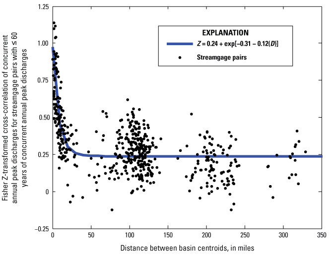
Relation between Fisher Z-transformed cross-correlation of logarithms of annual peak discharges and distance between basin centroids for streamgage pairs in the Hawaiʻi regional skew study, using data through water year 2020. Abbreviations: ≤, less than or equal to; Z, Fisher Z-transformation; exp, natural exponential function; D, distance between basin centroids, in miles.
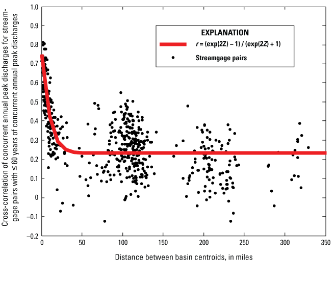
Relation between un-transformed cross-correlation of logarithms of annual peak discharges and distance between basin centroids for streamgage pairs in the Hawaiʻi regional skew study, using data through water year 2020. Abbreviations: ≤, less than or equal to; r, sample correlations; exp, natural exponential function; Z, Fisher Z-transformation.
Regional Skew Model
Seventeen basin characteristics—BASINPERIM, BSLDEM10M, CENTROIDX, CENTROIDY, COMPRAT, CSL10_85, DRNAREA, ELEV, ELEVMAX, RELIEF, RELRELF, PERM24IN, LFPORNE, I60M2Y, I6H500Y, I48H500Y, and PRECIP—were tested as covariates in the B–WLS/B–GLS analysis of regional skew (see table 3 in the main body of this report) (the “LFPORNE” basin characteristic—although not used in the body of the report or listed in table 3—describes the mean orientation of the longest flow path within the drainage basin, relative to the predominant trade winds from the northeast). Three candidate models were considered:
-
(1) a constant model using at-site skews from streamgages in all 10 flood regions in Hawaiʻi (table 1.1, app. 1; see also figs. 2–6 in the main body of this report);
-
(2) unique constant models for windward (2, 4, 6, and 8) and leeward (1, 3, 5, 7) regions; and
-
(3) a constant model for windward regions and a model incorporating the basin slope (BSLDEM10M) as a covariate for leeward regions.
The second and third options offered no treatment of regional skew for flood regions 9 and 10 (Island of Hawaiʻi), which did not have a clear windward/leeward orientation and had an insufficient number of streamgages from which to develop a unique constant model. Therefore, the first candidate model, a constant model of regional skew (GR) for all of Hawaiʻi, −0.157, was selected (table 3.2).
Table 3.2.
Regional skew model for Hawaiʻi and model performance metrics.[Standard deviations are in parentheses.is the model error variance. ASEV: Average sampling error variance. AVPnew: Average variance of prediction for a new site. Pseudo : Describes the fraction of the variability in the true skews explained by each model (Gruber and others, 2007).]
A good regional skew model will have the smallest possible model error variance, , and largest possible pseudo-. A constant model does not explain variability in the at-site skews, so the pseudo-, which describes the estimated fraction of the variability in the at-site skews explained by the model (Gruber and others, 2007; Parrett and others, 2011), is zero. The posterior mean of the model error variance, , is 0.194. The average sampling error variance, ASEV, is 0.0184 and represents the average error in the regional skew for the streamgages in the dataset. The average variance of prediction at a new site, AVPnew, is 0.212, which is equivalent to the MSE of the regional skew (MSER) and corresponds to an effective record length (ERL) of 36 years. The updated GR (−0.157) and MSER (0.212), and ERL are an improvement upon and supersede GR (−0.05), MSER (0.302), and ERL (17 years) from the generalized skew map in Bulletin 17B (Interagency Advisory Committee on Water Data, 1982), which was used in the previous study (Oki and others, 2010).
Diagnostic Statistics for Bayesian Weighted Least Squares/Bayesian Generalized Least Squares Regression
To evaluate how well a regression model fits a regional hydrologic dataset, diagnostic statistics have been developed (Griffis, 2006; Gruber and others, 2007). A pseudo analysis of variance (pseudo ANOVA) was conducted for the constant model of regional skew in Hawaiʻi (table 3.3). The pseudo ANOVA shows how much of the variation in the observed skews can be explained by the regional model, and how much of the variation in residuals can be attributed to model error and sampling error, respectively. Difficulties arise in determining these quantities. The model errors cannot be resolved because the values of the sampling errors, , for each site, i, are not known. However, the total sampling error sum of squares can be described by its mean value, . Because there are n equations, the total variation because of the model error for a model with k parameters has a mean equal to; thus, the residual variation attributed to the sampling error is, and the residual variation attributed to the model error is. This division of the variation in the observations is referred to as a pseudo ANOVA because the contributions of the three sources of error are estimated or constructed, rather than being determined from the residuals and the model predictions, while also ignoring the effect of correlation among the sampling errors.
Table 3.3.
Pseudo analysis of variance (ANOVA) table for the regional skew model of Hawaiʻi.[Abbreviations: k, number of estimated regression parameters not including the constant; n, number of observations (streamgages) used in regression; , model error variance of a constant model; , model error variance of a model with weak k regression parameters and a constant; NA, not applicable; , variance of the estimated sample skew at site i; EVR, error variance ratio; MBV*, misrepresentation of the beta variance; pseudo , fraction of variability in the true skews explained by each model (Gruber and others, 2007); %, percent; , regression constant from WLS analysis; WLS, weighted least squares; GLS, generalized least squares; WT, the transformation of W; , covariance matrix; , the (k×n) matrix of weights determined by WLS analysis; v, the (n×1) vector of 1s; ]
For a model with no parameters other than the mean (a constant skew model), the estimated model error variance, , describes all of the anticipated variation in , where is the mean of the estimated station sample skews; thus, the total expected sum of squares variation because of model error, , and because of sampling error, in expectation should equal . The expected sum of squares attributed to a regional skew model with k parameters should then equal , because the sum of the model error variance and the variance explained by the model must sum to. The constant model does not have any explanatory variables, thus the variation attributed to the models is 0 and k = 0.
The ratio of the average sampling error variance to the model error variance is called the error variance ratio (EVR) and is a diagnostic statistic used to evaluate if a simple OLS regression is sufficient or if a more sophisticated WLS or GLS analysis is appropriate. Generally, an EVR greater than 0.20 indicates that the sampling variance is not negligible when compared to the model error variance, suggesting the need for a WLS or GLS regression analysis. The EVR is calculated as:
The EVR for the constant model is 0.7. The sampling variability in the at-site skew was larger than the error in the regional model; thus, an OLS model that neglects sampling error in the at-site skew might not provide a statistically reliable analysis of the data. Given the variation of record lengths among streamgages, it was important to use a WLS or GLS analysis to evaluate the final precision of the model, rather than a simpler OLS analysis.
The misrepresentation of the beta variance (MBV) is a diagnostic statistic that is used to determine whether a WLS regression is sufficient or a GLS regression is appropriate to determine the precision of the estimated regression parameters (Griffis, 2006; Veilleux, 2011). The MBV describes the error produced by a WLS regression analysis in its evaluation of the precision of , which is the estimator of the constant , because the covariance among the estimated at-site skews, , generally has its greatest impact on the precision of the constant term (Stedinger and Tasker, 1985). If the MBV is substantially greater than 1, then a GLS error analysis should be employed. The MBV is calculated as
whereMBV for the constant model was 6.9. This is a large value, indicating that the cross-correlation among the at-site skew estimates affected the precision with which the regional skew could be estimated. If a WLS analysis were used to estimate the precision of the constant, the variance would be underestimated by a factor of 6.9; moreover, a WLS model would underestimate the variance of prediction, given that the sampling error in the constant term was sufficiently large to make an appreciable contribution to the average variance of prediction.
Leverage and Influence
Leverage and influence diagnostics statistics can be used to identify rogue observations and to effectively address lack of fit when estimating skew coefficients. Leverage identifies those streamgages in the analysis where the observed values have a large effect on the fitted (or predicted) values (Hoaglin and Welsch, 1978). Generally, leverage takes into consideration whether an observation, or explanatory variable, is unusual, and thus likely to have a large effect on the estimated regression coefficients and predictions. Unlike leverage, which highlights points that have the ability or potential to affect the fit of the regression, influence attempts to describe those points that have an unusual impact on the regression analysis (Belsley and others, 1980; Cook and Weisberg, 1982; Tasker and Stedinger, 1989). An influential observation is one with an unusually large residual that has a disproportionate effect on the fitted regression. Influential observations often have high leverage. Detailed descriptions of the equations used to determine leverage and influence for a B–WLS/B–GLS analysis can be found in Veilleux (2011) and Veilleux and others (2011).
No streamgages in the regional skew analysis exhibited high leverage (greater than 0.016). The differences in leverage values for the constant model reflect the variation in record lengths among streamgages. Four streamgages exhibited high influence (Cook’s D greater than 0.032) and thus had an unusual impact on the fitted regression (table 3.4).
Table 3.4.
Streamgages with high influence on the regional skew model for Hawaiʻi.[High influence is defined as Cook's D values greater than 4/n (or 4/124=0.032). Each of the 124 streamgages in the regional skew study was assigned a ranking value from 1 to 124, signifying its relative rank, where a rank of 1 corresponds to the largest positive value in each category. The table is sorted from largest to smallest influence (Cook's D). Abbreviations: USGS, U.S. Geological Survey; PRL, pseudo effective record length; MSE, mean squared error]
References Cited
Belsley, D.A., Kuh, E., and Welsch, R.E., 1980, Regression diagnostics—Identifying influential data and sources of collinearity: Hoboken, New Jersey, John Wiley & Sons, Inc., 300 p. [Also available at https://doi.org/10.1002/0471725153.]
Cohn, T.A., Lane, W.L., and Baier, W.G., 1997, An algorithm for computing moments-based flood quantile estimates when historical flood information is available: Water Resources Research, v. 33, no. 9, p. 2089–2096, accessed October 1, 2019, at https://pubs.er.usgs.gov/publication/70019489.
Cohn, T.A., Lane, W.L., and Stedinger, J.R., 2001, Confidence intervals for expected moments algorithm flood quantile estimates: Water Resources Research, v. 37, no. 6, p. 1695–1706. [Also available at https://doi.org/10.1029/2001WR900016.]
England, J.F., Jr., Cohn, T.A., Faber, B.A., Stedinger, J.R., Thomas, W.O., Jr., Veilleux, A.G., Kiang, J.E., and Mason, R.R., Jr., 2019, Guidelines for determining flood flow frequency—Bulletin 17C (ver. 1.1, May 2019): U.S. Geological Survey Techniques and Methods, book 4, chap. B5, 148 p., accessed April 1, 2020, at https://doi.org/10.3133/tm4B5.
Feaster, T.D., Gotvald, A.J., and Weaver, J.C., 2009, Magnitude and frequency of rural floods in the Southeastern United States, 2006—Volume 3, South Carolina: U.S. Geological Survey Scientific Investigations Report2009–5156, 226 p. [Also available at https://pubs.usgs.gov/sir/2009/5156/.]
Gotvald, A.J., Feaster, T.D., and Weaver, J.C., 2009, Magnitude and frequency of rural floods in the southeastern United States, 2006—Volume 1, Georgia: U.S. Geological Survey Scientific Investigations Report2009–5043, 120 p. [Also available at https://pubs.usgs.gov/sir/2009/5043/.]
Gruber, A.M., Reis, D.S., Jr., and Stedinger, J.R., 2007, Models of regional skew based on Bayesian GLS regression, in Kabbes, K.C., ed., Proceedings of the 2007 World Environmental and Water Resources Congress—Restoring our natural habitat, Tampa, Florida, May 15–18, 2007: Reston, Virginia, American Society of Civil Engineers, 10 p., accessed October 3, 2019, at https://doi.org/10.1061/40927(243)400.
Gruber, A.M., and Stedinger, J.R., 2008, Models of LP3 regional skew, data selection, and Bayesian GLS regression, in Babcock, R.W., and Walton, R., eds., World Environmental and Water Resources Congress 2008—Ahupua'a—Proceedings of the congress, Honolulu, Hawai'i, May 12–16, 2008: Reston, Virginia, American Society of Civil Engineers, p. 5575–5584. [Also available at https://doi.org/10.1061/40976(316)563.]
Lamontagne, J.R., Stedinger, J.R., Berenbrock, Charles, Veilleux, A.G., Ferris, J.C., and Knifong, D.L., 2012, Development of regional skews for selected flood durations for the Central Valley Region, California, based on data through water year 2008: U.S. Geological Survey Scientific Investigations Report 2012–5130, 60 p. [Also available at https://pubs.usgs.gov/sir/2012/5130/.]
Martins, E.S., and Stedinger, J.R., 2002, Cross correlations among estimators of shape: Water Resources Research, v. 38, no. 11, p. 34-1 to 34-7. [Also available at https://doi.org/10.1029/2002WR001589.]
Oki, D.S., Rosa, S.N., and Yeung, C.W., 2010, Flood-frequency estimates for streams on Kaua‘i, O‘ahu, Moloka‘i, Maui, and Hawai‘i, State of Hawai‘i: U.S. Geological Survey Scientific Investigations Report 2010–5035, 121 p., accessed February 10, 2020, at https://doi.org/10.3133/sir20105035.
Parrett, C., Veilleux, A.G., Stedinger, J.R., Barth, N.A., Knifong, D.L., and Ferris, J.C., 2011, Regional skew for California, and flood frequency for selected sites in the Sacramento–San Joaquin River Basin, based on data through water year 2006: U.S. Geological Survey Scientific Investigations Report2010–5260, 94 p. [Also available at https://doi.org/10.3133/sir20105260.]
Reis, D.S., Jr., Stedinger, J.R., and Martins, E.S., 2005, Bayesian generalized least squares regression with application to the log Pearson type 3 regional skew estimation: Water Resources Research, v. 41, no. 10, W10419, 14 p. [Also available at https://doi.org/10.1029/2004WR003445.]
Stedinger, J.R., and Tasker, G.D., 1985, Regional hydrologic analysis—1. Ordinary, weighted, and generalized least squares compared: Water Resources Research, v. 21, no. 9, p. 1421–1432. [Also available at https://doi.org/10.1029/WR021i009p01421.]
Stedinger, J.R., and Cohn, T.A., 1986, Flood frequency analysis with historical and paleoflood information: Water Resources Research, v. 22, no. 5, p. 785–793. [Also available at https://doi.org/10.1029/WR022i005p00785.]
Stedinger, J.E., and Griffis, V.W., 2008, Flood frequency analysis in the United States—Time to update: Journal of Hydrologic Engineering, v. 13, no. 4, p. 199–204. [Also available at https://doi.org/10.1061/(ASCE)1084-0699(2008)13:4(199).]
Tasker, G.D., 1978, Flood frequency analysis with a generalized skew coefficient: Water Resources Research, v. 14, no. 2, p. 373–376. [Also available at https://doi.org/10.1029/ WR014i002p00373.]
Tasker, G.D., and Stedinger, J.R., 1986, Regional skew with weighted LS regression: Journal of Water Resources Planning and Management, v. 112, no. 2, p. 225–237. [Also available at https://doi.org/10.1061/(ASCE)0733-9496(1986)112:2(225).]
Tasker, G.D., and Stedinger, J.R., 1989, An operational GLS model for hydrologic regression: Journal of Hydrology, v. 111, no. 1–4, p. 361–375. [Also available at https://doi.org/10.1016/0022-1694(89)90268-0.]
Veilleux, A.G., Stedinger, J.R., and Eash, D.A., 2012, Bayesian WLS/GLS regression for regional skewness analysis for regions with large crest stage gage networks, in Loucks, E.D., ed., Proceedings of the World Environmental and Water Resources Congress 2012—Crossing boundaries, Albuquerque, New Mexico, May 20–24, 2012: Reston, Virginia, American Society of Civil Engineers, p. 2253–2263.
Veilleux, A.G., Stedinger, J.R., and Lamontagne, J.R., 2011, Bayesian WLS/GLS regression for regional skewness analysis for regions with large cross-correlations among flood flows, in Beighley, R.E., II, and Killgore, M.W., eds., Proceedings of the World Environmental and Water Resources Congress 2011—Bearing knowledge for sustainability, Palm Springs, California, May 22–26, 2011: Reston, Virginia, American Society of Civil Engineers, p. 3103–3123.
Veilleux, A.G., and Wagner, D.M., 2019, Methods for estimating regional skewness of annual peak flows in parts of the Great Lakes and Ohio River Basins, based on data through water year 2013: U.S. Geological Survey Scientific Investigations Report 2019–5105, 26 p., accessed February 1, 2020, at https://doi.org/10.3133/sir20195105.
Veilleux, A.G., and Wagner, D.M., 2021, Methods for estimating regional skewness of annual peak flows in parts of eastern New York and Pennsylvania, based on data through water year 2013: U.S. Geological Survey Scientific Investigations Report 2021–5015, 38 p., accessed February 1, 2020, at https://doi.org/10.3133/sir20215015.
Weaver, J.C., Feaster, T.D., and Gotvald, A.J., 2009, Magnitude and frequency of rural floods in the Southeastern United States, through 2006—Volume 2, North Carolina: U.S. Geological Survey Scientific Investigations Report2009–5158, 111 p. [Also available at https://pubs.usgs.gov/sir/2009/5158/.]
Appendix 4. Magnitude, Variance, and Prediction Intervals of Annual Exceedance Probability Floods for Selected Streamgages in the State of Hawaiʻi
Magnitude, variance, and prediction intervals of annual exceedance probability discharges for selected streamgages in Kauaʻi, Oʻahu, Molokaʻi, Maui, and Hawaiʻi, State of Hawaiʻi.
[Table 4.1 is available in .xlsx and .cvs file formats at https://doi.org/10.3133/sir20235014.]
Conversion Factors
U.S. customary units to International System of Units
Temperature in degrees Fahrenheit (°F) may be converted to degrees Celsius (°C) as follows: °C = (°F – 32) / 1.8.
Datums
Vertical coordinate information is referenced to mean sea level.
Horizontal coordinate information is referenced to North American Datum of 1983 (NAD 83).
Altitude, as used in this report, refers to distance above the vertical datum.
For more information concerning the research in this report, contact the
Director, Pacific Islands Science Center
U.S. Geological Survey
1845 Wasp Blvd., B176
Honolulu, HI 96818
https://www.usgs.gov/centers/pacific-islands-water-science-center
Manuscript approved on February 7, 2023
Publishing support provided by the U.S. Geological Survey
Science Publishing Network, Tacoma Publishing Service Center
Edited by Jeff Suwak
Layout and design by Yanis X. Castillo
Illustration support by Luis Menoyo
Disclaimers
Any use of trade, firm, or product names is for descriptive purposes only and does not imply endorsement by the U.S. Government.
Although this information product, for the most part, is in the public domain, it also may contain copyrighted materials as noted in the text. Permission to reproduce copyrighted items must be secured from the copyright owner.
Suggested Citation
Mitchell, J.N., Wagner, D.M., and Veilleux, A.G., 2023, Magnitude and frequency of floods on Kauaʻi, Oʻahu, Molokaʻi, Maui, and Hawaiʻi, State of Hawaiʻi, based on data through water year 2020: U.S. Geological Survey Scientific Investigations Report 2023–5014, 66 p. plus 4 appendixes, https://doi.org/10.3133/sir20235014.
ISSN: 2328-0328 (online)
Study Area
| Publication type | Report |
|---|---|
| Publication Subtype | USGS Numbered Series |
| Title | Magnitude and frequency of floods on Kauaʻi, Oʻahu, Molokaʻi, Maui, and Hawaiʻi, State of Hawaiʻi, based on data through water year 2020 |
| Series title | Scientific Investigations Report |
| Series number | 2023-5014 |
| DOI | 10.3133/sir20235014 |
| Publication Date | March 27, 2023 |
| Year Published | 2023 |
| Language | English |
| Publisher | U.S. Geological Survey |
| Publisher location | Reston, VA |
| Contributing office(s) | Pacific Islands Water Science Center |
| Description | Report: vii, ; 8 Tables; 3 Data Releases |
| Country | United States |
| State | Hawaii |
| Other Geospatial | Kauaʻi, Oʻahu, Molokaʻi, Maui, Hawaiʻi |
| Online Only (Y/N) | Y |
| Additional Online Files (Y/N) | Y |