

Potentiometric Surfaces (2013, 2015), Groundwater Quality (2010–15), and Water-Level Changes (2011–13, 2013–15) in the Sparta-Memphis Aquifer in Arkansas
Links
- Document: Report (8.23 MB) , HTML , XML
- Plates:
- Plate 1 (3.90 MB pdf) - Potentiometric surface map for the Sparta-Memphis aquifer in Arkansas, 2013
- Plate 2 (3.77 MB pdf) - Potentiometric surface map for the Sparta-Memphis aquifer in Arkansas, 2015
- Plate 3 (2.99 MB pdf) - Water-level change map for the Sparta-Memphis aquifer in Arkansas 2011−13
- Plate 4 (2.95 MB pdf) - Water-level change map for the Sparta-Memphis aquifer in Arkansas 2013−15
- Appendixes:
- Appendix 1 (xlsx) - Water-Level Data Collected From Wells Screened in the Sparta-Memphis Aquifer in Arkansas, January–May 2013
- Appendix 1 (csv)
- Appendix 2 (xlsx) - Water-Level Data Collected From Wells Screened in the Sparta-Memphis Aquifer in Arkansas, January–June 2015
- Appendix 2 (csv)
- Appendix 4 (xlsx) - Wells and Differences in Water-Levels From 2011 To 2013 in the Sparta-Memphis Aquifer in Arkansas
- Appendix 4 (csv)
- Appendix 5 (xlsx) - Wells and Differences in Water-Levels From 2013 To 2015 in the Sparta-Memphis Aquifer in Arkansas
- Appendix 5 (csv)
- Data Releases:
- USGS data release - Potentiometric surface dataset of the Sparta-Memphis aquifer in Arkansas, January 2013 - May 2013 (ver. 1.2, June 2021)
- USGS data release - Datasets for the 2015 potentiometric surface and water-level changes (2011–2013, 2013–2015) in the Sparta-Memphis aquifer, in Arkansas
- NGMDB Index Page: National Geologic Map Database Index Page (html)
- Download citation as: RIS | Dublin Core
Acknowledgments
The authors would like to thank the Arkansas Department of Agriculture-Natural Resources Division, Arkansas Geological Survey, Natural Resources Conservation Service, Union County Water Conservation Board for providing funding to conduct this study. The authors would also like to extend their gratitude to numerous persons who contributed valuable time assisting in site reconnaissance and the various data collection efforts.
Abstract
The Sparta-Memphis aquifer, present across much of eastern Arkansas, is the second most used groundwater resource in the State, with the Mississippi River Valley alluvial aquifer being the primary groundwater resource. The U.S. Geological Survey, in cooperation with Arkansas Department of Agriculture-Natural Resources Division, Arkansas Geological Survey, Natural Resources Conservation Service, Union County Water Conservation Board, and the Union County Conservation District, collects groundwater data across the Sparta-Memphis aquifer extent in Arkansas. This report presents water-level data for measurements conducted during two time periods, January–May 2013 and January–June 2015, and discusses water-level altitude changes for the 2011–13 and 2013–15 periods in the Sparta-Memphis aquifer. Accompanying water-level data in this report include groundwater-quality data for the period 2010–15 in the Sparta-Memphis aquifer. Groundwater data can guide ongoing and future groundwater-monitoring efforts and inform management of the aquifers in Arkansas.
Water levels measured at 306 wells from January to May 2013 and 273 wells from January to June 2015 are graphically presented as potentiometric-surface maps. Measurements from 2011, 2013, and 2015 were used in the construction of 2011–13 and 2013–15 water-level change maps. Select long-term hydrographs are included in the report to illustrate water-level changes at the local scale.
Water-level data show the influence of climate, pumping, and conservation and management efforts on groundwater levels. With respect to climate, the study area experienced extreme drought conditions between January 2011 and December 2012. The proximate effects of drought—increased evapotranspiration, decreased recharge, and increased irrigation needs—resulted in water-level declines that were particularly notable in the northern and central portions of the study area.
Groundwater sampled in 2010–15 from 148 wells completed in the Sparta-Memphis aquifer was analyzed for specific conductance, pH, chloride (Cl) concentration, and bromide (Br) concentration. In 2015, groundwater-quality data from 103 wells completed in the Sparta-Memphis aquifer had a median specific conductance of 356 microsiemens per centimeter at 25 degrees Celsius and a median Cl concentration of 9.5 milligrams per liter (mg/L). The data show two areas of higher Cl (greater than 10 mg/L) and higher Br (greater than 0.5 mg/L) concentrations in Union, Calhoun, and Bradley Counties in southern Arkansas and Monroe and Phillips Counties in eastern-central Arkansas. A Cl and Br mixing model indicates the two regions of wells may have different sources of higher salinity. In the greater Union County area, water in most wells may be a mixture of recharge or precipitation and higher salinity groundwater from the Nacatoch aquifer. Water in wells in eastern-central Arkansas may be sourced from aquifers having a higher Cl concentration (and thus, also a higher Cl-to-Br ratio).
Introduction
The Sparta-Memphis aquifer is regionally referred to as the “Middle Claiborne aquifer of the Mississippi Embayment aquifer system” (Miller, 2000; Renken, 1998) and encompasses an area of approximately 20,324 square miles of which 38 percent is in Arkansas. The study area, defined as the Sparta-Memphis aquifer extent in Arkansas, is approximately bounded to the west by the “Fall Line,” a transitional zone between Paleozoic rocks of the Interior Highlands physiographic division and unconsolidated Cenozoic strata of the Coastal Plain physiographic province, which the Sparta-Memphis aquifer is contained in (Fenneman, 1938; Fenneman and Johnson, 1946). To the north, east, and south, the study area is bounded by the Missouri State line, the Mississippi River, and the Louisiana State line, respectively, all of which the full extent of the aquifer actually extends beyond (fig. 1).
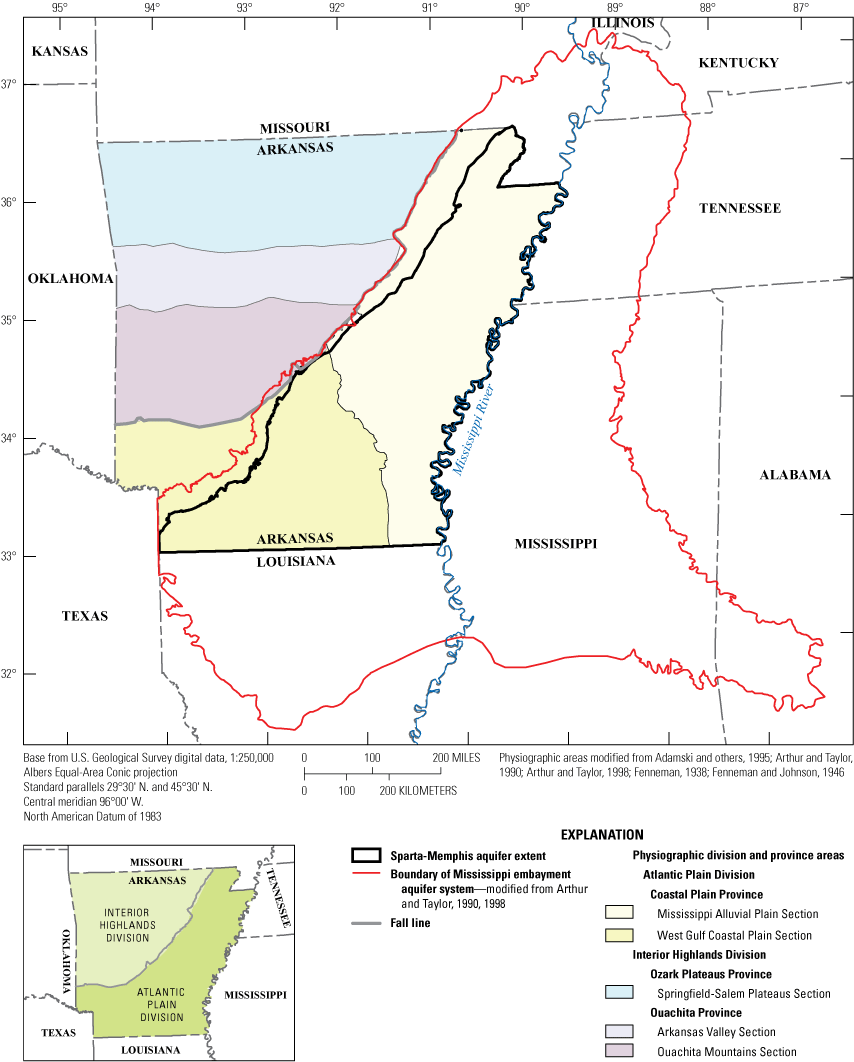
The study areas’ physiographic division, physiographic province, physiographic sections, Mississippi Embayment aquifer system boundary line, and Sparta-Memphis aquifer extent in Arkansas.
Arkansas groundwater withdrawal data indicate the Sparta-Memphis aquifer is the second most used groundwater resource in Arkansas, with the Mississippi River Valley alluvial (MRVA) aquifer being the most used aquifer in Arkansas (Kresse and others, 2014). The Sparta-Memphis aquifer has primarily been used for industry and public water supply, but the aquifer increasingly has been used for irrigation (McKee and Hays, 2002). Clark and others (2011) reported an average of about 170 million gallons per day (Mgal/d) was pumped from the Sparta-Memphis aquifer in 2005. Groundwater withdrawals from the aquifer in Arkansas have increased while water levels have declined, well yields have decreased, and water quality has degraded (Kresse and others, 2014). In the Grand Prairie critical groundwater area, an area of intensive agricultural water use historically met by withdrawals from the MRVA aquifer, pumping changes have caused water levels in the MRVA aquifer to decline to a degree that has curtailed use of groundwater from the aquifer. Moreover, the recent, increasing use of the Sparta-Memphis aquifer as an alternate agricultural supply is causing greater water-level declines in that aquifer as well. In contrast, conservation efforts have led to a long-term recovery in groundwater levels in Union County located in the South Arkansas critical groundwater area (fig. 2), where measures implemented in 2001 to decrease groundwater withdrawals have resulted in considerable water-level increases that have continued, even during drought periods. As a result, Federal and State agencies have worked to improve groundwater monitoring and groundwater policy and management approaches to protect the Sparta-Memphis aquifer and ensure continued, sustainable use of this resource. Continual aquifer assessment, modeling, planning, and management efforts are data intensive. To address these monitoring needs, the U.S. Geological Survey (USGS), in cooperation with Arkansas Department of Agriculture-Natural Resources Division (ADA–NRD), Arkansas Geological Survey, Natural Resources Conservation Service, Union County Water Conservation Board (UCWCB), and Union County Conservation District collect data on groundwater levels, water quality, and water use as part of ongoing efforts that provide data for effective management of groundwater resources in Arkansas. These data have driven the designation of critical groundwater areas (CGWAs) in accordance with the Arkansas Water Plan (Arkansas Department of Agriculture-Natural Resources Division, 1975; Arkansas Department of Agriculture-Natural Resources Division, 1990; Arkansas Department of Agriculture-Natural Resources Division, 2014): the South Arkansas CGWA for the Sparta-Memphis aquifer in 1996, the Grand Prairie CGWA for the Sparta-Memphis and MRVA aquifers in 1998, the Cache CGWA for the Sparta-Memphis and MRVA aquifers in 2009, and the Phillips County CGWA for the MRVA aquifer in 2015 (fig. 2). CGWAs are areas determined by ADA–NRD to have significant groundwater depletion and (or) water-quality degradation that compels the State to direct resources toward supporting improved and sustainable management (Arkansas Natural Resources Commission, 2015).
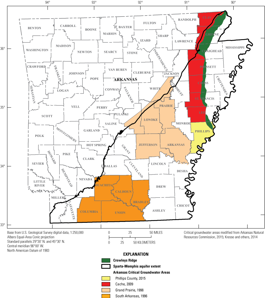
Arkansas’ four critical groundwater areas that overlap the study area.
Potentiometric-surface maps are one of several tools available to groundwater scientists, planners, and managers that aid understanding of the character and status of aquifers. In particular, these maps provide a graphical presentation of water-level data and give an indication of the status of water storage in an aquifer, the economic viability of extracting water, and when compared with past potentiometric-surface maps, information on changes in groundwater storage in time and space. Water-level and water-quality data presented in this report are a continuation of data presented by Kresse and others (2014) and Schrader (2014). Kresse and others (2014) evaluated water-level data from 1921 through 2009, water-quality data from approximately 1950 through 2010, and water-use data from 1965 through 2010. Schrader (2014) discussed Sparta-Memphis aquifer groundwater levels and water quality and presents a 2007–11 water-level-change map. This report presents Sparta-Memphis aquifer potentiometric-surface maps for 2013 (pl. 1) and 2015 (pl. 2), water-level-change maps for the 2011–13 period (pl. 3), and the 2013–15 period (pl. 4), and groundwater-quality data and analysis for 2010–15.
This report presents and analyzes potentiometric surfaces created from water-level data for measurements conducted during two time periods, January–May 2013 and January–June 2015, and discusses water-level altitude changes for the 2011–13 and 2013–15 periods in the Sparta-Memphis aquifer. Accompanying water-level data presented and analyzed in this report include groundwater-quality data for the 2010–15 period in the Sparta-Memphis aquifer.
Hydrogeologic Section
The study area is located within the areal extent of the Mississippi Embayment aquifer system (fig. 1) and contains the Sparta Sand and Memphis Sand of the Claiborne Group (fig. 3). Together, these units form the Sparta-Memphis aquifer, a term used to describe a sequence of groundwater-productive (the ability for a formation to store and transmit water), hydraulically connected sands that are often separated by silts and clays (Kresse and others, 2014; Miller, 2000; Pugh and others, 1998; Renken, 1998). Together, the Sparta Sand and Memphis Sand range in thickness from 0 to 900 feet (ft) and are present in approximately one-third of southeastern Arkansas (Pugh and others, 1998). The hydraulic properties of the Sparta-Memphis aquifer vary, with the highest transmissivity values exhibited by the thickest sand intervals (Kresse and others, 2014; Payne, 1968). Additional information on the hydraulic properties of the Sparta-Memphis aquifer have been discussed in previous studies (Brahana and Broshears, 1989; Hosman and others, 1968; Kresse and others, 2014; Plebuch and Hines, 1969; Pugh, 2008).
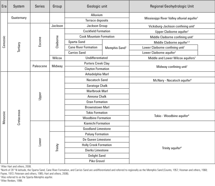
Correlated Tertiary and Quaternary geologic and hydrogeologic units of the Mississippi Embayment aquifer system and Mississippi River Valley alluvial aquifer, Arkansas, modified from Kresse and others (2014).
The Sparta Sand of the Mississippi Embayment aquifer system is overlain by the Cockfield and Cook Mountain Formations of the Claiborne Group and underlain by the Cane River Formation of the Claiborne Group (fig. 3). These formations are mostly fine grained and relatively impermeable across most of central and southeastern Arkansas and act to confine the Sparta-Memphis aquifer. The Sparta-Memphis aquifer is unconfined where the Sparta Sand crops out in southern Arkansas (Hosman, 1982; Hosman and others, 1968; Petersen and others, 1985) (fig. 4), generally at and just east of its western extent along the Fall Line. In outcrop areas, the Sparta-Memphis aquifer receives recharge from direct infiltration and streams (Kresse and others, 2014). East of the outcrop area, the Sparta Sand dips generally eastward and transitions to a confined aquifer (Kresse and others, 2014; McKee and Hays, 2002); the Sparta-Memphis aquifer receives recharge where it subcrops in the subsurface by way of leakage from adjacent aquifers. In northeastern Arkansas, the Sparta Sand is rarely observed in outcrop but subcrops under the Mississippi River Valley alluvial aquifer (fig. 4). In this area, the Sparta-Memphis aquifer and MRVA aquifer are hydraulically connected, making this an important Sparta-Memphis aquifer recharge area (Broom and Lyford, 1981; Hosman and others, 1968; Kresse and others, 2014). In east-central Arkansas at an approximate latitude of 35 degrees north, the Cane River Formation transitions lithologically from predominantly clay to predominantly sand moving south to north. In this area, the Cane River Formation, the underlying Carrizo Sand of the Claiborne Group, and the overlying Sparta Sand form a single sand unit whose components are indistinguishable and referred to regionally as the Memphis Sand (Counts, 1957; Hart and others, 2008; Hosman and others, 1968; Miller, 2000; Payne, 1972; Petersen and others, 1985; Renken, 1998).
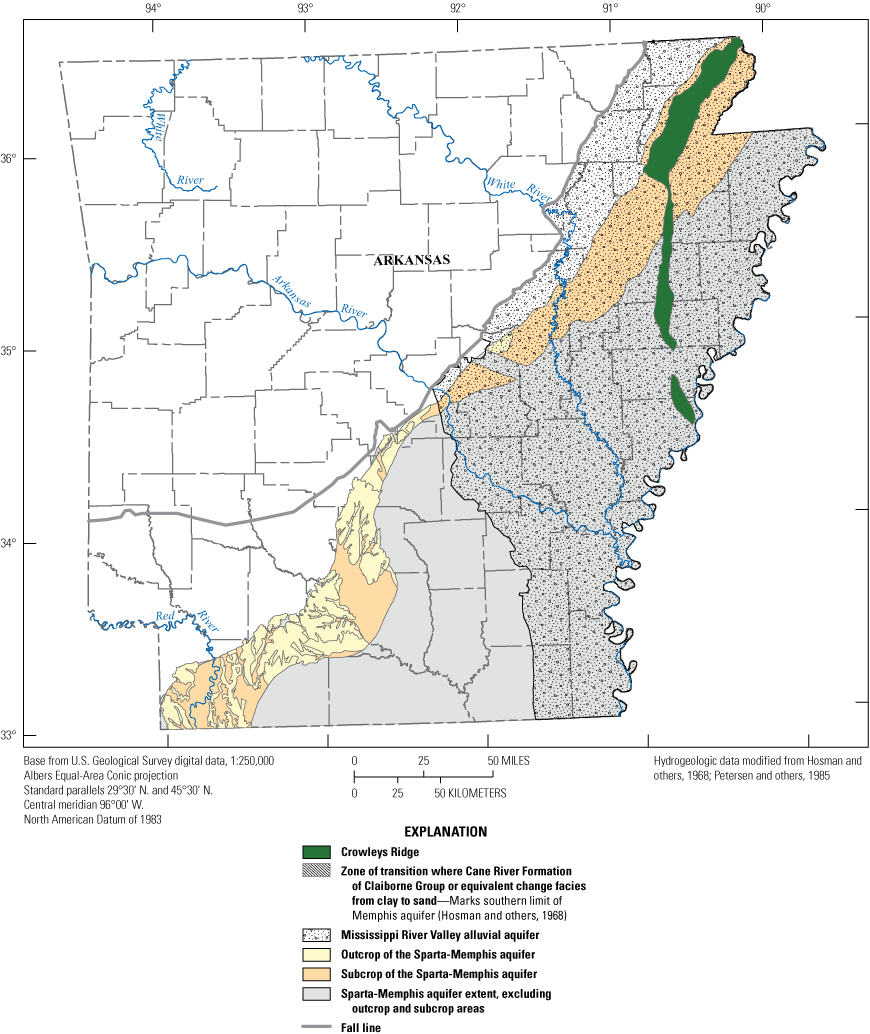
The extent of the Mississippi River Valley alluvial aquifer, Sparta-Memphis aquifer extent, and the outcrop and subcrop of the Sparta-Memphis aquifer, in Arkansas.
Methods
The USGS, in cooperation with the ADA–NRD, Arkansas Geological Survey, Natural Resources Conservation Service, UCWCB, and Union County Conservation District, collect water-level and water-quality data for the Sparta-Memphis aquifer biennially (during odd years), generally starting in January or February. The Union County Conservation District measures Sparta-Memphis aquifer groundwater levels on behalf of the UCWCB in the south Arkansas counties of Bradley, Calhoun, Columbia, Ouachita, and Union on a rotating quarterly basis for over 100 wells and monthly basis for wells equipped with automated data loggers. Groundwater levels are collected following USGS groundwater technical procedures presented in Cunningham and Schalk (2011) using a graduated steel tape or an electric water-level indicator. Tapes are calibrated and accurate to within 0.01 ft. Well locations have previously been verified using a Global Positioning System. Groundwater data are uploaded into and are publicly available through the USGS National Water Information System (U.S. Geological Survey, 2017a). Water-level data undergo a rigorous quality-assurance protocol to reduce possible errors from nonrepresentative water-level measurements caused by recent or nearby pumping, data not representative of water levels in the aquifer system, and measurement errors.
Water-level measurements in feet below land surface were converted to water-level altitude, in feet above the North American Vertical Datum of 1988 (NAVD 88), for construction of potentiometric-surface maps. Well altitudes originally reported in reference to the National Geodetic Vertical Datum of 1929 were converted to NAVD 88 for consistency using data obtained from the National Elevation Dataset (U.S. Geological Survey, 2017b).
Potentiometric-Surface Maps
Potentiometric-surface maps are conceptual surfaces representing the areal distribution of hydraulic head, which is the level to which water would rise in a well completed at any given location in a confined aquifer (Fetter, 2001). The potentiometric surface of a confined aquifer is analogous to the water-table surface in an unconfined aquifer. Water-level altitudes derived from a potentiometric map should not be used to determine the absolute water-level altitude or depth to water at any given location because of variable hydrologic properties and water-level change over time. Potentiometric surfaces indicate general direction of flow under isotropic conditions, with flow moving perpendicular to the lines of equal hydraulic head and in the direction of decreasing hydrologic gradient (Fetter, 2001). A potentiometric-surface map provides approximate water-level altitudes for an area at a given time, general direction and gradient of groundwater flow, and information on areas of water-level decline—all of which are useful information for water-management planners.
Two potentiometric-surface maps were constructed: a 2013 Sparta-Memphis aquifer potentiometric-surface map (pl. 1) constructed using water-level data collected from 306 wells measured from January through May 2013 (app. 1) (Nottmeier, 2018; U.S. Geological Survey, 2017a) and a 2015 Sparta-Memphis aquifer potentiometric-surface map (pl. 2) constructed using water-level data collected from 275 wells measured from January through June 2015 (app. 2) (Nottmeier and others, 2023; U.S. Geological Survey, 2017a). A single, representative measurement was selected to include in potentiometric-map construction for wells for which quarterly or monthly data were available. Measurement selection was based on the timing of the biennial USGS water-level measurement run, which is timed to collect roughly synoptic, spring-season measurements and is concluded before water users begin to increase groundwater pumping during the drier summer period.
Surface-water altitudes in streams were used to provide additional data control for the outcrop areas of the Sparta-Memphis aquifer. Perennial streams represent the intersection of the groundwater table with land surface. Stream data were obtained from the USGS National Hydrography Dataset (U.S. Geological Survey, 2018). The “select by location” tool in ArcMap 10.5 (Esri, 2018) was used to determine perennial stream reaches that lay within the outcrop areas.
Sparta-Memphis aquifer potentiometric-surfaces were then generated from select well and stream locations using the interpolation method, topo to raster, in ArcMap 10.5 (Esri, 2017b). The “topo-to-raster” tool is specifically designed to help create hydrologically correct digital elevation models while imposing constraints to ensure a connected drainage structure and correct representation of the resulting surface (Esri, 2017b). After the raster surface was generated, 20-ft contours were created using the ArcMap 10.5 “spatial analyst contour” tool (Esri, 2017a), which is available through the ArcGIS 3D Analyst toolbox and creates a line-feature class of contours from the raster surface. ArcMap 10.5 topo-to-raster and contouring processes are a rapid way to interpolate data, but computer programs may neither consider hydrologic connections between groundwater and surface water, nor changes in aquifer hydraulic properties. For these reasons, contours were adjusted manually as needed to account for distribution of water-level controls to represent the potentiometric surface more accurately.
Water-Level Change Maps
Water-level change maps for the Sparta-Memphis aquifer were constructed to provide point-to-point comparison with wells measured in 2011, 2013, and 2015 (pls. 3 and 4). Only wells that were measured more than two times and therefore had paired measurements (such as 2011–13 or 2013–15) were used to construct the water-level change maps. The 2011–13 water-level change map presents data from 261 wells (pl. 3), whereas the 2013–15 water-level change map presents data from 241 wells (pl. 4). Water-level differences were calculated by subtracting 2011 water-level measurements, in feet below land surface, from the 2013 water-level measurements, in feet below land surface, and the 2013 water-level measurements, in feet below land surface, from 2015 water-level measurements, in feet below land surface. The water-level change maps show areas of water-level rise or decline across the Sparta-Memphis aquifer for the two periods represented.
Long-term hydrographs (minimum 25-year period of record) (app. 3) were selected for 22 individual wells to illustrate groundwater-level change at the local scale. These hydrographs are designated by letters “A” through “V” in appendix 3 and in the 2013 and 2015 data spreadsheets (apps. 1 and 2). The associated control points for the hydrographs are shown in red on the 2013 and 2015 potentiometric-surface maps (pls. 1 and 2). Collection of water-level data over one or more decades is required to compile a hydrologic record that encompasses the potential range of water-level fluctuations in an observation well and to track trends over time (Taylor and Alley, 2001). Long-term water-level data aid resource managers in understanding how groundwater level relates to fluctuations caused by variations in climatic conditions, land-use, or water-management practices. The availability of long-term water-level records greatly enhances the ability to forecast future water levels.
Groundwater Quality Sample Collection and Analysis
Groundwater-quality samples were collected from 148 wells screened in the Sparta-Memphis aquifer from 2010 to 2015 (fig. 5), generally during the summer and fall months. In 2015 (the focus of this report), groundwater-quality samples were collected from 103 wells screened in the Sparta-Memphis aquifer (fig. 5). Samples were analyzed for specific conductance, temperature, pH, chloride (Cl), and bromide (Br). Bromide analysis was only completed in 2012, 2014, and 2015. Water-quality data collection followed USGS National Field Manual procedures (U.S. Geological Survey, variously dated). Wells were purged prior to sampling by removing a minimum of three well-casing volumes of water, and field parameters (temperature, pH, and specific conductance) were monitored until measurements stabilized to ensure a representative sample was collected from the aquifer. Water-quality monitoring equipment was calibrated twice daily. In 2015, specific conductance was measured only at the USGS National Water Quality Laboratory in Denver, Colorado, for 32 out of 103 samples. Br and Cl samples were filtered in the field using 0.45-micrometer filters and analyzed at the National Water Quality Laboratory by inductively coupled plasma ion chromatography (Fishman and Friedman, 1985). All water-quality data presented in this report are accessible through the USGS National Water Information System database (U.S. Geological Survey, 2017a), which provides access to groundwater, surface-water, and water-quality data across the United States.
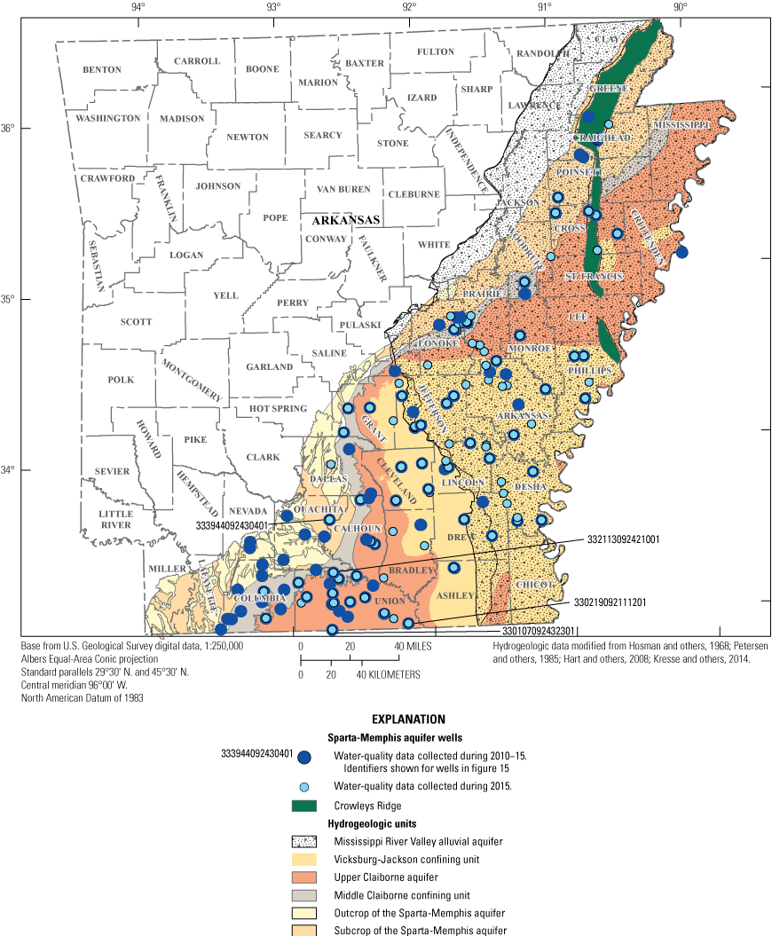
Sparta-Memphis aquifer wells sampled for water-quality during the 2010–15 sampling period. Hydrogeologic units that overlie the Sparta-Memphis aquifer are also shown for reference.
Quality Control
Quality-control (QC) field samples were collected and analyzed during the sampling events to assess the representativeness of the samples and potential for extraneous interference (or bias) in samples from field sample collection procedures. QC field samples included 111 replicates used to assess variability in field parameters, Cl and Br, as well as 13 blanks to assess potential bias in Cl or Br from extraneous sources. QC samples were collected following USGS National Field Manual procedures (U.S. Geological Survey, variously dated) and analyzed using the same laboratory and methods as the environmental samples. No Cl or Br detections were found in field blanks; Br blanks (n = 3) were less than the reporting limits of 0.03 and 0.01 milligram per liter (mg/L) and Cl blanks (n = 10) were less than the reporting limits of 0.12 (samples collected in 2010), 0.06 (samples collected from 2011 to 2013), and 0.02 mg/L (samples collected from 2014 to 2015). Variability in field parameters, Br, and Cl was low, as indicated by summary statistics of the standard deviation of paired environmental and field QC replicate samples (table 1). Of importance are the replicate samples collected for Br because of the generally small amounts of Br detected in groundwater samples. In general, variability in Br concentration was on the same order of magnitude as the reporting limits (table 1).
Table 1.
Summary statistics for the standard deviation of paired environmental and field quality-control replicate samples.[mg/L, milligram per liter; µS/cm at 25 °C, microsiemens per centimeter at 25 degrees Celsius; NA, not applicable]
Data Analysis
Water-quality data typically include results that are less than a reporting limit (indicated by a less than sign “<” in the data tables) and are termed “censored.” For this study, only Br included censored data, with two samples having concentrations less than the reporting limit of 0.01 mg/L and six samples having concentrations less than the reporting limit of 0.03 mg/L; there are two reporting limits because of changes in analytical procedures at the laboratory. To provide summary statistics and complete calculations of Cl to Br mass ratios, censored data were imputed using the robust regression on order statistics (ROS) method from Helsel (2012), which accounts for multiple reporting limits. In brief, in the robust ROS method, the probability of exceeding each reporting limit is calculated using the proportion of data that are equal to or above the reporting limit. Normal scores then are calculated separately for censored and uncensored data to build a regression between uncensored data normal scores and the log concentration. Finally, censored data are imputed using the regression equation and normal scores and retransformed to estimate concentrations for the censored data (Helsel, 2012). As cautioned by Helsel (2012, p. 83), “Estimated values produced for censored observations . . . should not be assigned to any individual sample.” Therefore, values imputed using the robust ROS method were used for calculations but were not reported for individual censored samples.
Conservative species, such as Cl and Br, can be used as tracers of the hydrologic cycle and to quantify mixing of water sources with different end-member concentrations (Davis and others, 1998). In particular, Cl and Cl-to-Br mass ratios have been used in groundwater studies to define typical compositions of potable groundwater across the United States (Davis and others, 2004) and to identify contamination of freshwater resources from anthropogenic sources, such as septic waste or oilfield brines, or natural sources such as mineralized groundwater from other aquifers (Davis and others, 1998; Katz and others, 2011). Both Br and Cl data were available for 130 samples; most samples were collected from different wells, with only seven wells that were resampled. All 130 samples were used in the mixing-model calculations.
For mixing models involving two conservative species (for example, Cl and Br) in two end-member groundwater sources, the proportion of one end member () in mixed groundwater (XM) is defined as follows (Eby, 2004):
whereA second conservative species in mixed groundwater (YM) is defined as follows:
whereWhen end-member concentrations are known and substantially different, the proportion of each end member ( and , or 1 − ) can be solved for.
Water Use
Water-use data for the United States have been reported by the USGS every 5 years since 1950 (U.S. Geological Survey, 2017a). Groundwater-use data in this report for Arkansas are from the USGS 5-year reports for 2010 (Maupin and others, 2014) and 2015 (Dieter and others, 2018). Data from these reports are compiled from various sources from each State and validated. In Arkansas, the ADA–NRD, in cooperation with the USGS, conducts an annual inventory of reported groundwater withdrawals by county for 10 categories: public supply, domestic (self-supplied), commercial (self-supplied), industrial (self-supplied), mining, livestock, aquaculture, irrigation, duck (hunting) clubs, and thermoelectric power generation (Pugh and Holland, 2015). Arkansas law requires that any nondomestic user of groundwater that has the potential to withdraw 50,000 gallons per day or more must report their annual water usage (Arkansas Department of Agriculture-Natural Resources Division, 2023). Water-use information for Arkansas may be found in the following reports and database: “Estimated Water Use in Arkansas, 2010” (Pugh and Holland, 2015), “Aquifers of Arkansas—Protection, Management, and Hydrologic and Geochemical Characteristics of Groundwater Resources in Arkansas” (Kresse and others, 2014), and USGS Lower Mississippi Gulf-Arkansas Water Use database, available at https://wise.er.usgs.gov/wateruse/.
Results—Controls on Water Levels and the Character of the Potentiometric-Surface Maps
Water levels are controlled by aquifer hydraulic characteristics, water input, and water output. The controls that are most temporally variable and therefore lie within the realm of groundwater management concern are the inputs, which are primarily dependent on climate (rainfall, humidity, and temperature) and vegetation/land cover, and outputs, which from the management perspective are primarily dependent on pumping.
Water-level altitudes in 306 wells measured for the 2013 potentiometric-surface map (pl. 1) ranged from 112 ft below to 445 ft above NAVD 88 (app. 1). Water-level altitudes in 275 wells measured for the 2015 potentiometric-surface map (pl. 2) ranged from 108 ft below to 447 ft above NAVD 88 (app. 2). Isopotential contours, showing a 20-ft water-level altitude interval generated from these data for the 2013 (pl. 1) and 2015 (pl. 2) potentiometric-surfaces (pl. 2), ranged from 100 ft below NAVD 88 in the South Arkansas CGWA to 440 ft above NAVD 88 in the aquifer outcrop area.
The 2013 and 2015 potentiometric-surface maps (pls. 1 and 2) show that the direction of groundwater flow generally is toward the south and southwest in the northern part of the Sparta-Memphis aquifer extent in Arkansas, and generally toward the southeast in the southern part of the study area; some minor topographic control on groundwater flow is apparent near Crowleys Ridge in the northern half of the study area and in the Sparta-Memphis aquifer outcrop area in the western part of the study area. Broad regional perturbations in these general patterns are centered on major cones of depression caused by groundwater pumping. A comparison of the 2013 and 2015 maps with the predevelopment potentiometric-surface map prepared by Fitzpatrick and others (1990) indicates that the recent potentiometric surface and groundwater-flow patterns across most of the Sparta-Memphis aquifer extent in Arkansas have been altered considerably by pumping.
A confined aquifer yields water to a pumping well by a decrease in pressure (equivalent to hydraulic head) in an area around the well known as the zone of influence; within this zone, hydraulic heads are measurably decreased, with the largest decreases observed near the well. This decrease in hydraulic heads is manifest as a depression in the potentiometric surface that is often conical in form and is termed a “cone of depression.” Greater amounts of water pumped over time result in greater drop in hydraulic head and an increasing zone of influence. Cones of depression centered on individual wells can grow and coalesce over time, resulting in regional cones of depression. These cones of depression alter, and even reverse, flow directions as compared to original, predevelopment conditions as the hydrologic system adjusts to provide water to pumping wells.
Two regional-scale cones of depression are indicated on both the 2013 and 2015 potentiometric-surface maps (pls. 1 and 2). One cone of depression is centered on a heavily pumped area in Jefferson County and the other is centered on a pumping center in Union County (Joseph, 2000; McKee and Hays, 2002). Arkansas has focused conservation and management resources on these two areas of regional decline using CGWA designations, the 1998 Grand Prairie CGWA, and the 1996 South Arkansas CGWA. No cone of depression is discernable at the 20-ft contour interval scale on either the 2013 or 2015 potentiometric-surface maps for the Cache CGWA or the Phillips County CGWA, but considerable water-level declines are observed on the 2011–13 water-level change map for these areas. Comparison of the 2011–13 and 2013–15 water-level change maps show the effect of groundwater withdrawals and climatic differences between the periods for drought, precipitation, and temperature.
The 2011–13 water-level change map (pl. 3) was constructed using data from 261 wells (app. 4); 146 of these wells exhibit declines ranging from –19.00 to –0.01 ft, and 115 exhibit rises ranging from 0.07 to 43.50 ft. Well 54 (app. 4) had the greatest decline (–19.00 ft) and well 56 (app. 4) had the greatest rise (43.50 ft). Both wells are located in Columbia County. In the Cache CGWA, 15 of 16 wells show declines, ranging from –3.76 to –1.39 ft (pl. 3). In the Phillips CGWA, all six wells also show declines, ranging from –17.76 to –1.14 ft. In the Grand Prairie CGWA, 52 of the 76 wells show declines, ranging from –9.35 to –0.07 ft, and 24 wells show rises, ranging from 0.21 to 14.47 ft. In the South Arkansas CGWA, 19 of the 71 wells show declines, ranging from –19.00 to –0.01 ft, and 71 wells show rises, ranging from 0.07 to 43.50 ft.
The 2013–15 water-level change map (pl. 4) was constructed using 241 wells (app. 5); 83 of these wells exhibit declines, ranging from –22.96 to –0.01 ft), and 158 wells exhibit rises, ranging from 0.04 to 16.89 ft. Well 35 in Bradley County had the greatest decline (–22.96 ft, app. 5), and well 119 in Jefferson County had the greatest rise (16.89 ft, app. 5). Of the nine wells located in the Cache CGWA, seven of the wells show water-level declines, ranging from –7.23 to –0.15 ft, and two wells show rises, ranging from 0.53 to 0.74 ft (pl. 4). In the Phillips CGWA, two of the seven wells show declines, ranging from –2.24 to –0.52 ft, and five wells show rises, ranging from 0.18 to 11.05 ft. In the Grand Prairie CGWA, 27 of the 71 wells show declines, ranging from –10.08 to –0.01 ft, and 44 wells show rises, ranging from 0.51 to 16.89 ft. In the South Arkansas CGWA, 30 of 92 wells exhibit declines, ranging from –22.96 to –0.01 ft, and 62 wells exhibit rises, ranging from 0.24 to 12.49 ft. Changes in groundwater level rise or declines can be affected over time by groundwater usage and climatic conditions.
The 2010, 5-year water-use report by Pugh and Holland (2015) lists groundwater withdrawals of 7,790 Mgal/d in Arkansas, with the Sparta-Memphis aquifer supplying 192 Mgal/d of that total (Kresse and others, 2014). Among the counties, groundwater use was greatest in Arkansas County (one of six counties located in the Grand Prairie CGWA) in 2010, with a county total of 540.08 Mgal/d. Of the groundwater withdrawals in Arkansas County, 56.71 Mgal/d was from the Sparta-Memphis aquifer (Pugh and Holland, 2015). Groundwater withdrawals from the Sparta-Memphis aquifer are also large in Jefferson County, which is also located in the Grand Prairie CGWA, with withdrawals of 43.49 Mgal/d reported for 2010 (Pugh and Holland, 2015). The primary use of groundwater from the Sparta-Memphis aquifer in Jefferson County was industrial, with 35.35 Mgal/d withdrawn in 2010 (Pugh and Holland, 2015). Industrial and public water supply have historically been the major Sparta-Memphis aquifer groundwater uses in the two regional cone-of-depression areas in the Grand Prairie CGWA, but over the years irrigation groundwater withdrawals from the Sparta-Memphis aquifer have increased because of groundwater declines and decreasing groundwater availability in the MRVA aquifer. This change in the source of groundwater for irrigation has occurred in other parts of Arkansas where the MRVA aquifer is used and is particularly apparent in the Grand Prairie CGWA.
The Grand Prairie CGWA is an area of intensive agricultural water use that historically has been supplied by withdrawals from the MRVA aquifer (Hays and Fugitt, 1999; Kresse and others, 2004). This aquifer has experienced water-level declines to a degree that has led to curtailed groundwater use from that aquifer; as a result, farmers have turned to the Sparta-Memphis aquifer as an alternate supply. Because the Sparta-Memphis aquifer is confined across most of Arkansas, it has only a fraction of the water storage of the MRVA aquifer. For this reason, water managers have expressed great concern regarding the sustainability of agricultural withdrawals from the Sparta-Memphis aquifer (Hays, 2001; McKee and Hays, 2002). Kresse and others (2014) reported that more water was used from the Sparta-Memphis aquifer for irrigation in Arkansas than for any other purpose as of 2010. Moreover, Arkansas was reported in 2015 as one of five States in the Nation to have 70 percent or more of its total fresh groundwater withdrawals used for irrigation (Dieter and others, 2018), with fresh groundwater defined as having less than 1,000 mg/L of dissolved solids. National total irrigation withdrawals were similar in 2010 and 2015, but notable changes were observed at the State level in Arkansas, Montana, and Wyoming (Dieter and others, 2018).
Climate Conditions From 2011 To 2015
Climatic conditions played a role in water-level changes between 2011 to 2015. On the 2013–15 water-level change map (pl. 4, app. 5), 83 of the total 241 wells in the study area show a water-level decline and 158 wells show a rise. In contrast, on the 2011–13 water-level change map (pl. 3, app. 4), 146 of the total 261 wells in the study area show a decline and 115 wells show a rise. Many wells showing water-level declines on the 2011–13 water-level change map (pl. 3) were in the northern and central part of the study area where the MRVA and Sparta-Memphis aquifers are hydraulically connected. The southern part of the study area was also experiencing a drought during 2011–13 (pl. 3), but water levels in wells located within the Union County cone of depression have generally risen since 2004, and intensive conservation efforts in the area led by the UCWCB have prevented the cone of depression from expanding (Schrader, 2009, 2014; Schrader and Jones, 2007).
The Palmer Drought Severity Index (PDSI) for the National Climatic Data Center divisions—namely, the northeast, central, east central, southeast, south central, and southwest, which encompasses the study area—show an average range as follows: 2011, –0.1 to –3.8; 2012, –1.0 to –3.4; 2013, –0.4 to 1.2; 2014, 0.2 to 1.7; 2015, 0.0 to 2.7 (table 2, fig. 6) (National Centers for Environmental Information, 2019). During 2011–15 the PDSI would classify this period as severe drought to moderate wet (table 3, fig. 6). The PDSI is an index formulated by Palmer (1965) that takes into account precipitation, potential and actual evapotranspiration, infiltration of water into a given soil zone, and runoff (American Meteorological Society, 2017). The PDSI builds on the work of Thornthwaite (1931, 1948) by adding soil depth zones to better represent regional change in soil water-holding capacity and movement between soil zones (American Meteorological Society, 2017; Palmer, 1965).
Table 2.
Summary of Palmer Drought Severity Index values for Arkansas’ National Climatic Data Center (NCDC) climate divisions in Arkansas from January 2011 to December 2015.[Modified from National Centers for Environmental Information (2019). More negative numbers on the Palmer Drought Severity Index indicate drought, more positive numbers indicate wetness. For the Palmer Drought Severity Index classification, see table 3; max, maximum; min, minimum]
Table 3.
Palmer Drought Severity Index (PDSI) classification.[Modified from National Centers for Environmental Information (2019). PDSI calculated from precipitation and temperature data, and available water content of soil]
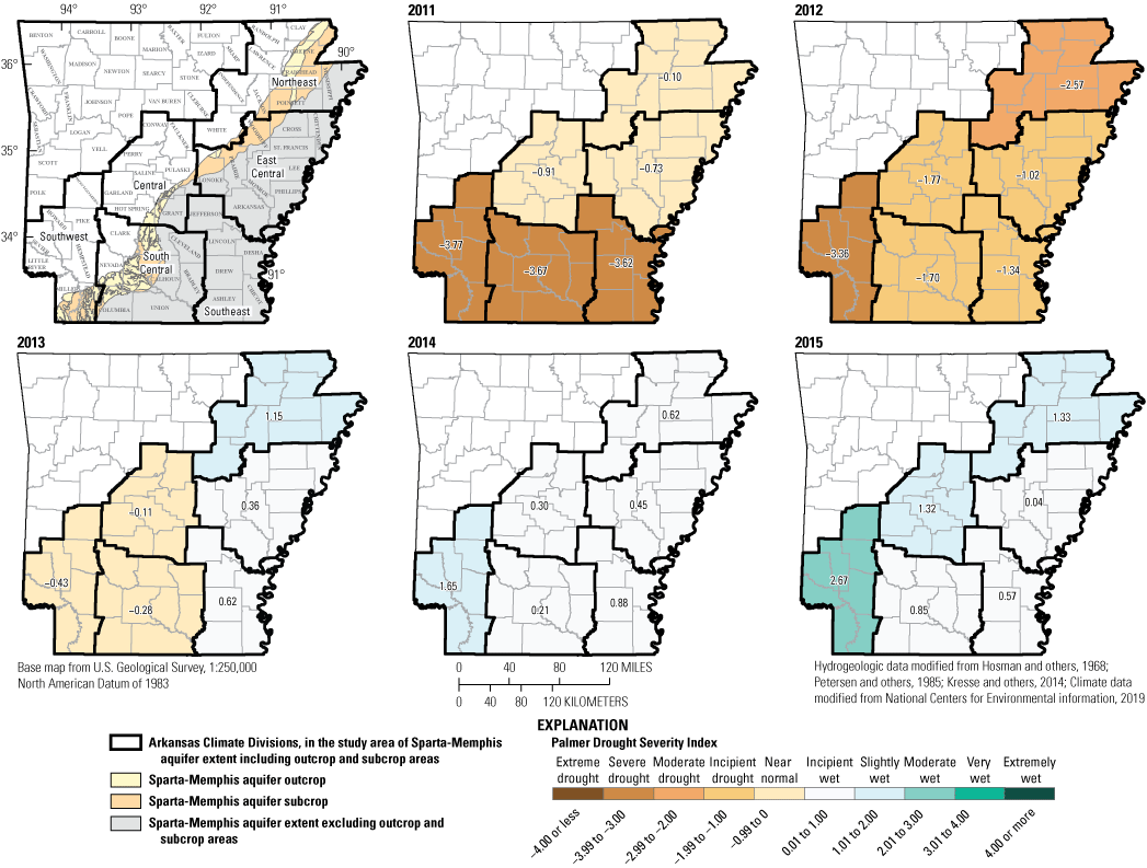
Annual average Palmer Drought Severity Index for select National Climatic Data Center (NCDC) climate divisions that include the area of the Sparta-Memphis aquifer extent in Arkansas, 2011–15.
The PDSI events between January 2011 and January 2013 that encompassed the study area begin to fluctuate between severe drought to near normal conditions (table 3; fig. 7A). It’s not until about March 2013 that the encompassed study area begins to see slightly wet to very wet conditions (table 3, fig. 7A). Although an increase in precipitation is indicated in some months during 2011–15 (fig. 7B), warmer temperatures prevailed during these times. During this period, the ranges of precipitation values for the climate divisions encompassing the study area were as follows: 2011, 32.4–69.0 inches (in.); 2012, 31.9–50.0 in.; 2013, 46.3–64.6 in.; 2014, 39.3–58.5 in.; 2015, 52.9–79.4 in. (table 4, fig. 8), and the ranges of average temperature values were as follows: 2011, 59.0–65.9 degrees Fahrenheit (°F); 2012, 61.0–66.5 °F; 2013, 56.8–63.1 °F; 2014, 56.2–62.2 °F; 2015, 59.0–64.8 °F (table 5, fig. 9) (National Centers for Environmental Information, 2019). Warmer air temperatures result in higher evapotranspiration rates, which in turn leads to decreased groundwater recharge and greater groundwater withdrawals for irrigation, both of which result in declining groundwater levels. Climate studies have shown that a warmer atmosphere will hold more moisture, often leading to fewer but more intense rainfall events (Carey, 2011; Trenberth, 2005, 2011), which can result in higher runoff/infiltration ratios over time, despite the possibility of longer dry spells between events. With fewer events and increased runoff/infiltration ratios, groundwater recharge will decrease.
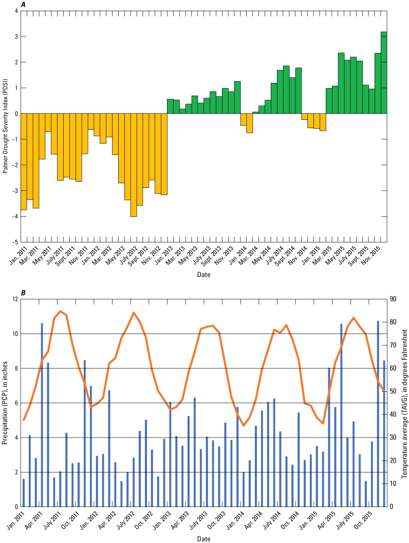
A, Palmer Drought Severity Index (PDSI) data from select National Climatic Data Center (NCDC) climate divisions where the study area encompasses and B, monthly total precipitation and temperature averages in degrees Fahrenheit for the select NCDC climate divisions where the study area encompasses, 2011–15.
Table 4.
Arkansas' county precipitation data from January 2011 to December 2015, for National Climatic Data Center (NCDC) climate divisions and counties in the Sparta-Memphis aquifer areal extent.[Data modified from National Centers for Environmental Information (2019)]
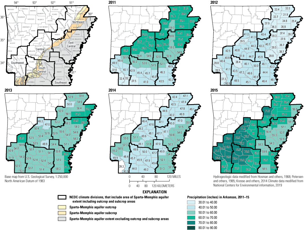
Arkansas' county precipitation data, in inches, from January 2011 to December 2015, for National Climatic Data Center (NCDC) divisions and area of Sparta-Memphis aquifer extent.
Table 5.
Arkansas' county average temperature data from January 2011 to December 2015, for National Climatic Data Center (NCDC) climate divisions and counties in the Sparta-Memphis aquifer areal extent.[Data modified from National Centers for Environmental Information (2019). °F, degree Fahrenheit]
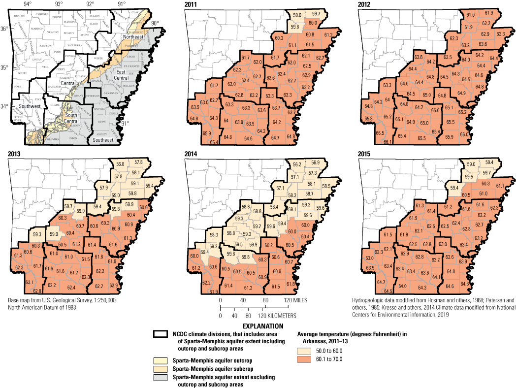
Arkansas' county annual average temperature data, in degrees Fahrenheit, from January 2011 to December 2015, for National Climatic Data Center divisions and area of Sparta-Memphis aquifer extent.
During drought conditions, groundwater withdrawals typically increase from the Sparta-Memphis and overlying MRVA aquifers. Drought related decreases in recharge to the Sparta-Memphis aquifer in the outcrop areas, coupled with increased pumping in the MRVA aquifer, also reduce water levels in the Sparta-Memphis aquifer. The combined effects of increased pumping from the MRVA aquifer and decreased recharge to the Sparta-Memphis aquifer can be expected to result in accentuated groundwater declines during drought, particularly in areas where these aquifers are hydraulically connected and leakage from the MRVA aquifer is an important source of recharge to the Sparta-Memphis aquifer (Craighead, Poinsett, Cross, Woodruff, Lonoke, and Phillips Counties).
The rises indicated on the 2013–15 water-level change map could be due to drought conditions beginning to dissipate as the study area began to receive increasing rainfall (National Weather Service, 2018a). During June 2014, parts of the study area experienced extreme rainfall events and flooding, including Woodruff, St. Francis, Prairie, Crittenden, and Monroe Counties. Areas of Woodruff County experienced precipitation amounts ranging from 7.5 to 10.3 in., causing some cities and thousands of acres of farmland to flood along the Cache River (National Weather Service, 2018b). The statewide average precipitation of 10.6 in. in May 2015 was the second largest May precipitation amount on record (National Weather Service, 2018c). The increased rainfall caused decreased withdrawals from the Sparta-Memphis aquifer, allowing water levels to rise.
Water-Quality Conditions From 2010 To 2015
Water-quality data will be discussed for the period 2010–15 and separately for 2015 to better place the results from 2015 in context. Specific conductance in the Sparta-Memphis aquifer for 322 wells measured from 2010 through 2015 ranged from 29 to 1,380 microsiemens per centimeter at 25 degrees Celsius (µS/cm at 25 °C) with a median of 366 μS/cm, and in 103 wells measured in 2015 ranged from 35 to 1,220 μS/cm, with a median of 356 μS/cm (table 6). Median specific conductance values generally were between approximately 350 and 450 μS/cm each year (fig. 10). Values of pH ranged from 4.6 to 9.8 for the period 2010–15 and for 2015, with a median of 8.2 for measurements over the period 2010–15 and 8.1 in 2015 (table 6). Median pH values generally were between 7.5 and 8.8 each year (fig. 11). Cl concentrations ranged from 1.2 to 230 mg/L for the period 2010–15, and from 1.2 to 218 mg/L for 2015, with a median of 13.2 mg/L for the period 2010–15 and 9.5 mg/L for 2015 (table 6). Median Cl values generally were less than 15 mg/L each year (fig. 12). Br concentrations ranged from < 0.01 to 1.16 mg/L for the period 2012–15 and for 2015, with a median of 0.06 mg/L for both periods (table 6). Median Br values generally were less than 0.1 mg/L each year (fig. 13).
Table 6.
Summary statistics for water-quality data for 2010–15 and 2015.[µS/cm at 25 °C, microsiemens per centimeter at 25 degrees Celsius; mg/L, milligram per liter]
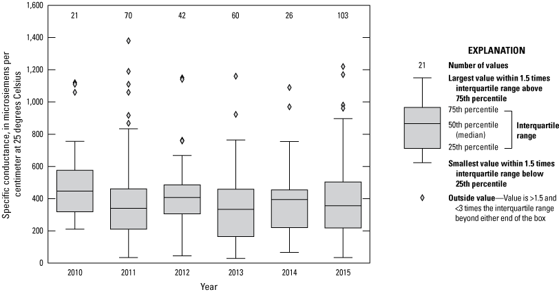
Specific conductance by year in the Sparta-Memphis aquifer in Arkansas, 2010–15.
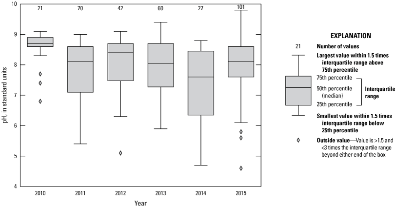
pH by year in the Sparta-Memphis aquifer in Arkansas, 2010–15.
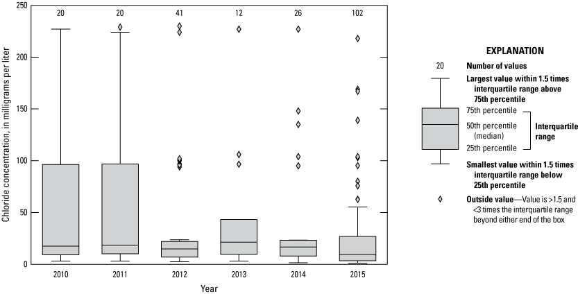
Chloride concentration by year in the Sparta-Memphis aquifer in Arkansas, 2010–15.
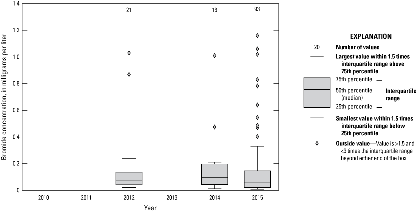
Bromide concentration by year in the Sparta-Memphis aquifer in Arkansas, 2010–15.
Water-quality parameters varied spatially across the Sparta-Memphis aquifer in Arkansas (fig. 14). Concentration of specific conductance and Cl and Br were generally lower in approximately the same south-central region of the study area compared to other areas of the aquifer, being less than approximately 225 μS/cm, 5 mg/L Cl, and 0.03 mg/L Br, respectively. In general, pH was most acidic (lowest) in the outcrop and westernmost parts of the subcrop area of the Sparta-Memphis aquifer and most basic (highest) in the eastern parts of Arkansas and near the Mississippi River (fig. 14).
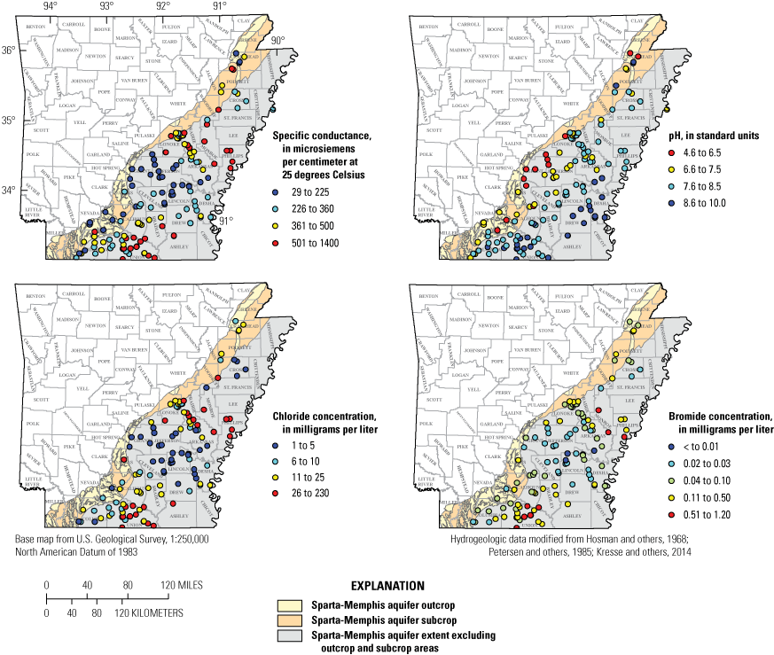
Specific conductance, pH, chloride concentration, and bromide concentration across the Sparta-Memphis aquifer in Arkansas collected from 2010 to 2015.
The 5-year water-quality datasets for specific conductance, pH, Cl, and 3-year dataset for Br presented in the boxplots (figs. 10–13) should not be used to interpret trends in groundwater quality, because the relatively short period analyzed is insufficient to confidently establish trends. Additionally, because of the spatial variability in water-quality parameters (fig. 14) and temporal differences in wells sampled, variability in water-quality data from year to year may be related to the different populations of wells sampled.
Long-term water-quality datasets from the same locations provide a robust mechanism to assess changes in groundwater quality over time. Four well sites in the South Arkansas CGWA were sampled multiple times between 2010 and 2015 (fig. 15). Water-quality parameters and constituents for each of these sites were relatively stable, except for a decrease in pH over time at site 333944092430401.
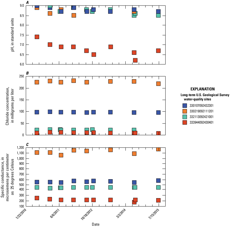
Water-quality data for pH, chloride concentration, and specific conductance, 2010–15. Location of wells shown on figure 5.
Groundwater quality in the Sparta-Memphis aquifer is generally good per drinking water standards (Kresse and others, 2014), although some areas exhibit relatively high salinity (Broom and others, 1984) and spatially variable specific conductance (Schrader, 2014). Groundwater chloride concentrations above 10 mg/L, higher than elsewhere in the Sparta-Memphis aquifer extent, were measured in clustered areas in Union, Calhoun, and Bradley Counties in southern Arkansas and in eastern-central Arkansas, in the Grand Prairie region (Lonoke, Prairie, and Arkansas Counties) and Monroe and Phillips Counties (fig. 14). Elevated specific conductance and Br concentrations were measured in the same areas (fig. 14). The zones of higher Cl, Br, and specific conductance observed during 2010–15 are the same areas noted by Kresse and others (2014) and studied historically to understand the source of salinity in the Sparta-Memphis aquifer (Broom and others, 1984; Hosman and others, 1968).
The sources of salinity in the Sparta-Memphis aquifer have been of interest because of concerns about water quality limiting the usability of groundwater resources. In the Grand Prairie region of Lonoke, Prairie, and Arkansas Counties, saline groundwater is observed in both the Sparta-Memphis aquifer and the overlying MRVA aquifer (Morris and Bush, 1986). Saline groundwater in the Sparta-Memphis aquifer is attributed to upward flow of more mineralized water from deeper aquifers, such as the Carrizo Sand (Hosman and others, 1968) or the underlying Nacatoch aquifer (Morris and Bush, 1986). Deeper, saline groundwater is able to migrate into the Sparta-Memphis aquifer because (1) the Cane River Formation undergoes a facies change such that clays thin and sands thicken as the Sparta Sand transitions to the Memphis Sand (figs. 3 and 4) (indicated by the northern extent of the Lower Claiborne confining unit) with corresponding increases in permeability, and (2) hydraulic heads are high enough in the underlying Carrizo and Nacatoch aquifers to induce upward flow of groundwater. Furthermore, the upward flow of saline groundwater from the Sparta-Memphis aquifer into the MRVA aquifer is hypothesized to occur along faults or where confining units, such as the Vicksburg-Jackson confining unit are thin or absent (Kresse and Clark, 2008; Kresse and others, 2014; Paul and others, 2018). The source of more saline groundwater in the Sparta-Memphis aquifer in the areas of Union, Calhoun, and Bradley Counties in southern Arkansas is less studied and less understood than in other parts of the system (Kresse and others, 2014). Broom and others (1984) hypothesized that the source of salinity (in Union County) was from restricted flushing of groundwater in a down-dropped graben within the Sparta-Memphis aquifer and not from surficial brine contamination or upward movement of more saline groundwater from deeper units. Although Br and Cl concentrations indicate that deeper units, such as the Carrizo Sand or Nacatoch aquifer, could be the sources of saline groundwater in the Sparta-Memphis aquifer in Union County, hydraulic heads were not sufficiently high in the Nacatoch aquifer to induce upward flow (Broom and others, 1984). The spatial extent of elevated Cl concentrations has increased over time, however, and was hypothesized to increase spatially as a result of groundwater pumping from the Sparta-Memphis aquifer (Broom and others, 1984).
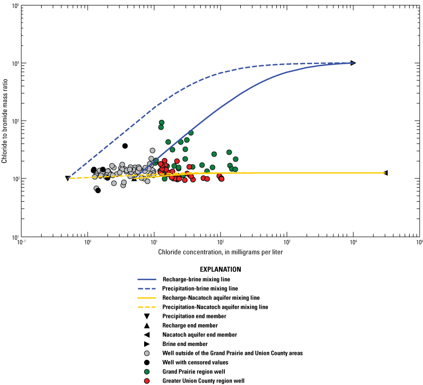
A mixing model using Cl and Cl-to-Br mass ratios of high-salinity groundwater sources and freshwater from either a precipitation or recharge source was constructed to further investigate groundwater compositions in the Sparta-Memphis aquifer (fig. 16). High salinity end members included (1) groundwater from the Nacatoch aquifer having an average Cl concentration of 30,000 mg/L, Br concentration of 240 mg/L, and Cl-to-Br mass ratio of 125 (Morris and Bush, 1986); and (2) a hypothetical brine composition—used by Davis and others (1998) to investigate groundwater mixing across the United States—having a Cl concentration of 10,000 mg/L, Br concentration of 1 mg/L, and Cl-to-Br mass ratio of 10,000. The hypothetical freshwater end members were precipitation and recharge where precipitation (Cl concentration of 0.5 mg/L and Br concentration of 0.005 mg/L) will undergo evaporation such that recharge water is slightly concentrated in these constituents (Cl concentration of 5 mg/L and Br concentration of 0.05 mg/L), but the mass ratio of 100 is the same (Davis and others, 1998).
Chloride and bromide with mixing lines.
Sparta-Memphis aquifer groundwater generally plots between mixing lines that represent the low Cl concentration end members of either recharge or precipitation and a high Cl concentration end member of either Nacatoch aquifer groundwater (low Cl-to-Br mass ratio) or a theoretical brine (high Cl-to-Br mass ratio) (fig. 16). Much of the groundwater data lie on mixing lines between precipitation or recharge and Nacatoch aquifer groundwater (fig. 16). Because of the differences in possible sources of salinity between the Grand Prairie and greater Union County areas, wells with Cl concentrations greater than 10 mg/L (fig. 14) are plotted by region and divided into two groups: one north (Grand Prairie) of and the other south (Union County) of approximately latitude 34 °N (fig. 5). Wells from the two areas plot along slightly different mixing lines, with wells in the greater Union County area plotting closer to the recharge/precipitation-Nacatoch mixing lines and wells in the Grand Prairie region plotting along a mixing line with a possible brine end member. Censored Br data are also shown on the plot because Br concentrations were imputed and can, therefore, affect the exact position of the Cl-to-Br mass ratio. Important observations can be drawn from these mixing lines: (1) Cl and Br mixing curves are consistent with deeper units underlying the Sparta-Memphis aquifer within the Mississippi Embayment (such as the Nacatoch aquifer) being a source of salinity and (2) another source of salinity, or specifically high Cl concentration, is needed to explain the Sparta-Memphis aquifer groundwater compositions with higher Cl-to-Br mass ratios (or greater Cl concentrations compared to Br concentrations). Although the greater Union County area wells generally plot along the recharge/precipitation-Nacatoch aquifer mixing lines, the hydraulic gradient observed by Broom and others (1984) between the Sparta-Memphis aquifer and the Nacatoch aquifer was downward rather than upward, as would be required to induce flow from the Nacatoch aquifer; therefore, information about hydraulic heads in adjacent aquifers, groundwater-flow directions, and groundwater chemistry may better constrain the sources of salinity in the Sparta-Memphis aquifer. In general, a correlation between Cl and Br is observed, with higher Cl concentrations occurring with higher Br concentrations (fig. 17), which implies that the possible brine end member is sourced from a single, dominant source of Cl (Davis and others, 1998).
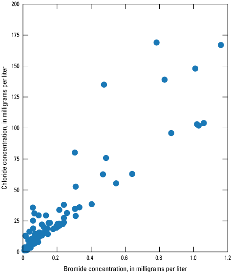
Chloride versus bromide concentrations in Sparta-Memphis aquifer wells in Arkansas.
Summary
The Sparta Sand and Memphis Sand of the Claiborne Group together form the Sparta-Memphis aquifer, a sequence of groundwater productive (the ability for a formation to store and transmit water), hydraulically connected sands that are present across most of the eastern one-third of Arkansas. Arkansas groundwater withdrawal data indicate the Sparta-Memphis aquifer is the second most used groundwater resource in Arkansas, with an average of about 170 million gallons per day pumped in 2005. The Sparta-Memphis aquifer is predominantly used for public and industrial supply, but over the years, irrigation groundwater withdrawals have increased because of water-level declines in the Mississippi River Valley alluvial (MRVA) aquifer. Increased groundwater withdrawals from the Sparta-Memphis aquifer have increased water-level declines, decreased well yields, and degraded water quality in the aquifer, which led to efforts by Federal and State agencies to improve groundwater monitoring and groundwater policy and management approaches. To address these needs, the U.S. Geological Survey, in cooperation with the Arkansas Department of Agriculture-Natural Resources Division, Arkansas Geological Survey, Natural Resources Conservation Service, Union County Water Conservation Board, and Union County Conservation District, collects data on groundwater levels, water quality, and water use as part of ongoing groundwater-monitoring efforts that provide data for effective aquifer management in Arkansas. Groundwater data from this ongoing study can be used to guide groundwater-monitoring efforts and provide information for State and Federal protection and management programs.
Potentiometric-surface maps of the Sparta-Memphis aquifer were prepared to illustrate 2013 and 2015 conditions. Water-level altitudes in 306 wells measured for the 2013 potentiometric-surface map ranged from 112 feet (ft) below to 445 ft above the North American Vertical Datum of 1988. Water-level altitudes in 275 wells measured for the 2015 potentiometric-surface map ranged from 108 ft below to 447 ft above the North American Vertical Datum of 1988. The 2013 and 2015 potentiometric-surface maps show that groundwater flow generally is toward the south and southwest in the northern part of the study area and toward the southeast in the southern part of the study area. The maps also indicate some minor topographic control on groundwater flow near Crowleys Ridge in the northern half of the study area and in the Sparta-Memphis aquifer outcrop area in the western part of the study area. Broad regional perturbations in these general patterns are centered on major cones of depression caused by groundwater pumping. Two regional-scale cones of depression are indicated on both the 2013 and 2015 potentiometric-surface maps. One cone of depression is centered on a heavily pumped area in Jefferson County and the other is centered on a heavily pumped area in Union County. Comparison of the 2013 and 2015 potentiometric surfaces with the predevelopment potentiometric-surface map indicates that groundwater-flow patterns across most of the Sparta-Memphis aquifer extent in Arkansas have been altered considerably by pumping.
Industrial and public water supply have historically been the major groundwater users in the two regional-scale cone-of-depression areas, and Arkansas has focused conservation and management resources in areas experiencing regional declines using critical groundwater area (CGWA) designations, including the Cache CGWA, Phillips County CGWA, Grand Prairie CGWA, and South Arkansas CGWA. The Grand Prairie CGWA is an area of intensive agricultural water use historically supplied by withdrawals from the MRVA aquifer. This aquifer has experienced water-level declines to a degree that has led to curtailed groundwater use from that aquifer; as a result, farmers have turned to the Sparta-Memphis as an alternate supply.
Water-level change maps for the Sparta-Memphis aquifer were constructed by comparing the periods 2011–13 and 2013–15. The 2011–13 water-level change map contains data from 261 wells, with 144 wells exhibiting declines ranging from –19.00 to –0.01 ft, and 115 exhibiting rises ranging from 0.07 to 43.50 ft. The 2013–15 water-level change map contains data from 241 wells, with 83 wells exhibiting declines ranging from –22.96 to –0.01 ft, and 158 wells exhibiting rises ranging from 0.04 to 16.89 ft. A comparison of the 2011–13 and 2013–15 water-level change maps shows the effect of groundwater withdrawals and climate differences between periods for selected areas.
Climatic conditions also play a role in water-level changes between 2011 and 2015. Data obtained from the National Climatic Data Center for Palmer Drought Severity Index, precipitation, and temperature show parts of Arkansas in an extreme drought in 2012. This drought began to dissipate in April of 2013 as the study area began to receive increasing rainfall.
Water-quality data were evaluated for selected wells screened in the Sparta-Memphis aquifer from 2010 through 2015. Water-quality constituents and parameters varied spatially across the Sparta-Memphis aquifer in Arkansas during the evaluation period, but groundwater quality across the extent of most of the aquifer is considered suitable for most uses, although groundwater in some areas exhibits relatively high salinity and high specific conductance. Specific conductance and chloride and bromide concentrations all were lower in approximately the same central region of the study area, whereas pH was most acidic in the subcrop and outcrop area of the Sparta-Memphis aquifer and most basic in eastern Arkansas and along the Mississippi River. Areas of higher specific conductance and chloride and bromide concentrations are present in Union, Calhoun, and Bradley Counties in southern Arkansas and the Grand Prairie region of Lonoke, Prairie, and Arkansas Counties in east-central Arkansas. Groundwater in wells in eastern-central Arkansas may be sourced from groundwater having a higher chloride concentration (and thus, a higher chloride-to-bromide ratio as well).
References Cited
Adamski, J.C., Petersen, J.C., Freiwald, D.A., and Davis, J.V., 1995, Environmental and hydrologic settings of the Ozark Plateaus study unit, Arkansas, Kansas, Missouri, and Oklahoma: U.S. Geological Survey Water-Resources Investigations Report 94–4022, 76 p., accessed July 1, 2016, at https://pubs.usgs.gov/wri/wri944022/WRIR94-4022.pdf.
American Meteorological Society, 2017, Palmer Drought Severity Index—AMS glossary: American Meteorological Society website, accessed September 14, 2020, at http://glossary.ametsoc.org/wiki/Palmer_drought_severity_index.
Arkansas Department of Agriculture-Natural Resources Division, 1975, Arkansas water plan 1975: Arkansas Department of Agriculture-Natural Resources Division, 270 p., accessed February 27, 2019, at https://www.agriculture.arkansas.gov/natural-resources/divisions/water-management/arkansas-water-plan/.
Arkansas Department of Agriculture-Natural Resources Division, 1990, Arkansas water plan 1990 update: Arkansas Department of Agriculture-Natural Resources Division, 95 p., accessed February 27, 2019, at https://www.agriculture.arkansas.gov/natural-resources/divisions/water-management/arkansas-water-plan/.
Arkansas Department of Agriculture-Natural Resources Division, 2014, Arkansas water plan 2014 update: Arkansas Department of Agriculture-Natural Resources Division, 16 p., accessed February 27, 2019, at https://www.agriculture.arkansas.gov/wp-content/uploads/2020/05/awp_eastern-arkansas_basin.pdf.
Arkansas Department of Agriculture-Natural Resources Division, 2023, Water-use registration: Arkansas Department of Agriculture-Natural Resources Division web page, accessed August 29, 2023, at https://www.agriculture.arkansas.gov/natural-resources/divisions/water-management/groundwater-protection-and-management-program/water-use-registration /.
Arkansas Natural Resources Commission, 2015, The facts about critical groundwater designation: Arkansas Natural Resources Commission fact sheet, accessed February 27, 2019, at https://www.agriculture.arkansas.gov/natural-resources/divisions/water-management/groundwater-protection-and-management-program/critical-groundwater-a reas/.
Arthur, J.K., and Taylor, R.E., 1990, Definition of the geohydrologic framework and preliminary simulation of ground-water flow in the Mississippi Embayment aquifer system, Gulf Coastal Plain, United States: U.S. Geological Survey Water-Resources Investigations Report 86–4364, 97 p., accessed December 17, 2018, at https://pubs.er.usgs.gov/publication/wri864364.
Arthur, J.K., and Taylor, R.E., 1998, Ground-water flow analysis of the Mississippi Embayment aquifer system, south-central United States: U.S. Geological Survey Professional Paper 1416–I, 59 p., 9 pls., accessed December 17, 2018, at https://pubs.er.usgs.gov/publication/pp1416I.
Broom, M.E., Kraemer, T.F., and Bush, W.V., 1984, A reconnaissance study of saltwater contamination in the El Dorado aquifer, Union County, Arkansas: U.S. Geological Survey Water-Resources Investigations Report 84–4012, 47 p., accessed January 5, 2018, at https://pubs.er.usgs.gov/publication/wri844012.
Broom, M.E., and Lyford, F.P., 1981, Alluvial aquifer of the Cache and St. Francis River Basins, northeastern Arkansas: U.S. Geological Survey Open-File Report 81–476, 55 p., accessed March 19, 2018, at https://pubs.er.usgs.gov/publication/ofr81476.
Carey, J., 2011, Global warming and the science of extreme weather: Scientific American, June 29, 2011, accessed January 29, 2020, at https://www.scientificamerican.com/article/global-warming-and-the-science-of-extreme-weather/.
Clark, B.R., Westerman, D.A., and Fugitt, D.T., 2011, Simulation of the effects of groundwater withdrawals on water-level altitudes in the Sparta aquifer in the Bayou Meto-Grand Prairie area of eastern Arkansas, 2007–37: U.S. Geological Survey Scientific Investigations Report 2011–5215, 9 p., accessed March 19, 2018, at https://pubs.er.usgs.gov/publication/sir20115215.
Counts, H.B., 1957, Ground water resources of parts of Lonoke, Prairie, and White Counties, Arkansas: Arkansas Geological and Conservation Commission WRC–5, 65 p., accessed September 10, 2020, at https://www.geology.arkansas.gov/docs/pdf/publication/water_circulars/Water-Resources-Circular-5_v.pdf.
Cunningham, W.L., and Schalk, C.W., 2011, Groundwater technical procedures of the U.S. Geological Survey: U.S. Geological Survey Techniques and Methods, book 1, chap. A1, 154 p., accessed January 5, 2018, at https://pubs.er.usgs.gov/publication/tm1A1.
Dieter, C.A., Maupin, M.A., Caldwell, R.R., Harris, M.A., Ivahnenko, T.I., Lovelace, J.K., Barber, N.L., and Linsey, K.S., 2018, Estimated use of water in the United States in 2015: U.S. Geological Survey Circular 1441, 65 p., accessed February 27, 2019, at https://pubs.er.usgs.gov/publication/cir1441.
Esri, 2017a, Contour: Esri, Inc., web page, accessed December 5, 2017, at http://pro.arcgis.com/en/pro-app/tool-reference/3d-analyst/contour.htm.
Esri, 2017b, How topo to raster works: Esri, Inc., web page, accessed December 5, 2017, at http://pro.arcgis.com/en/pro-app/tool-reference/3d-analyst/how-topo-to-raster-works.htm.
Esri, 2018, ArcGIS Desktop 10.5: Esri, Inc., software release, accessed March 13, 2018, at https://desktop.arcgis.com/en/.
Fenneman, N.M., and Johnson, D.W., 1946, Physical divisions of the conterminous United States: U.S. Geological Survey Map, scale 1:7,000,000, accessed October 30, 2018, at https://water.usgs.gov/lookup/getspatial?physio.
Fishman, M.J., and Friedman, L.C., 1985, Methods for determination of inorganic substances in water and fluvial sediments: U.S. Geological Survey Open-File Report 85–495, 709 p., accessed April 4, 2018, at https://pubs.er.usgs.gov/publication/ofr85495.
Fitzpatrick, D.J., Kilpatrick, J.M., and McWreath, H., 1990, Geohydrologic characteristics and simulated response to pumping stresses in the Sparta aquifer in east-central Arkansas: U.S. Geological Survey Water-Resources Investigations Report 88–4201, 50 p., 16 pls., accessed November 15, 2019, at https://pubs.er.usgs.gov/publication/wri884201.
Hart, R.M., Clark, B.R., and Bolyard, S.E., 2008, Digital surfaces and thicknesses of selected hydrogeologic units within the Mississippi Embayment Regional Aquifer Study (MERAS): U.S. Geological Survey Scientific Investigations Report 2008–5098, 33 p., accessed October 30, 2018, at https://pubs.usgs.gov/sir/2008/5098/.
Hays, P.D., 2001, Simulated response of the Sparta aquifer to outcrop area recharge augmentation, southeastern Arkansas: U.S. Geological Survey Water-Resources Investigations Report 2001–4039, 14 p., accessed September 14, 2020, at https://doi.org/10.3133/wri014039.
Hosman, R.L., Long, A.T., Lambert, T.W., Jeffery, H.G., and others, 1968, Tertiary aquifers in the Mississippi embayment: U.S. Geological Survey Professional Paper 448–D, 29 p., accessed September 9, 2020, at https://pubs.usgs.gov/pp/0448d/report.pdf.
Kresse, T.M., and Clark, B.R., 2008, Occurrence, distribution, sources, and trends of elevated chloride concentrations in the Mississippi River Valley Alluvial aquifer in southeastern Arkansas: U.S. Geological Survey Scientific Investigations Report 2008–5193, 35 p., accessed September 9, 2020, at https://pubs.er.usgs.gov/publication/sir20085193.
Kresse, T.M., Hays, P.D., Merriman, K.R., Gillip, J.A., Fugitt, D.T., Spellman, J.L., Nottmeier, A.M., Westerman, D.A., Blackstock, J.M., and Battreal, J.L., 2014, Aquifers of Arkansas—Protection, management, and hydrologic and geochemical characteristics of groundwater resources in Arkansas: U.S. Geological Survey Scientific Investigations Report 2014–5149, 334 p., accessed March 19, 2018, at https:/doi.org/10.3133/sir20145149.
McKee, P.W., and Hays, P.D., 2002, The Sparta aquifer—A sustainable water resources: U.S. Geological Survey Fact Sheet 111–02, 4 p., accessed March 19, 2018, at https://pubs.usgs.gov/fs/fs-111-02/.
Miller, J.A., 2000, Ground water atlas of the United States: U.S. Geological Survey Hydrologic Atlas 730, p. F1–F28, accessed January 23, 2018, at https://pubs.usgs.gov/ha/730f/report.pdf.
Morris, E.E., and Bush, W.V., 1986, Extent and source of saltwater intrusion into the alluvial aquifer near Brinkley, Arkansas, 1984: U.S. Geological Survey Water-Resources Investigations Report 85–4322, 123 p., accessed December 12, 2018, at https://doi.org/10.3133/wri854322.
National Centers for Environmental Information, 2019, Climate at a glance—Divisional mapping: National Oceanic and Atmospheric Administration website, accessed November 13, 2019, at https://www.ncdc.noaa.gov/cag/.
National Weather Service, 2018a, National temperature and precipitation maps—Temperature, precipitation, and drought: National Oceanic and Atmospheric Administration website, accessed October 18, 2018, at https://www.ncdc.noaa.gov/temp-and-precip/us-maps/12/201112?products[]=nationaltavgrank&products[]=nationalpcpnrank&products[]=regionaltavgrank&produc ts[]=regionalpcpnrank&products[]=statewidetavgrank&products[]=statewidepcpnrank&products[]=divisionaltavgrank&products[]=divisionalpcpnrank#us-maps-se lect.
National Weather Service, 2018b, NWS Little Rock, AR—Arkansas yearly climate summary (2014): National Oceanic and Atmospheric Administration website, accessed October 18, 2018, at https://www.weather.gov/lzk/2014.htm.
National Weather Service, 2018c, NWS Little Rock, AR—Arkansas yearly climate summary (2015): National Oceanic and Atmospheric Administration website, accessed October 18, 2018, at https://www.weather.gov/lzk/2015.htm.
Nottmeier, A.M., 2018, Potentiometric surface dataset of the Sparta-Memphis aquifer in Arkansas, January 2013 - May 2013 (ver. 1.2, June 2021): U.S. Geological Survey data release, https://doi.org/10.5066/F7X0657G.
Nottmeier, A.M., Knierim, K.J., and Hays, P.D., 2023, Datasets for the 2015 potentiometric surface and water-level changes (2011–2013, 2013–2015) in the Sparta-Memphis aquifer, in Arkansas: U.S. Geological Survey data release, https://doi.org/10.5066/F7N29W7H.
Palmer, W.C., 1965, Meteorological drought: U.S. Weather Bureau No. 45, 58 p., accessed September 14, 2020, at https://www.ncdc.noaa.gov/temp-and-precip/drought/docs/palmer.pdf.
Payne, J.N., 1968, Hydrologic significance of the lithofacies of the Sparta Sand in Arkansas, Louisiana, Mississippi, and Texas: U.S. Geological Survey Professional Paper 569–A, p. A1–A17, 14 pls., accessed March 19, 2018, at https://pubs.er.usgs.gov/publication/pp569A.
Payne, J.N., 1972, Hydrologic significance of lithofacies of the Cane River Formation or equivalents of Arkansas, Louisiana, Mississippi, and Texas: U.S. Geological Survey Professional Paper 569–C, p. C1–C17, 16 pls., accessed March 19, 2018, at https://pubs.er.usgs.gov/publication/pp569C.
Petersen, J.C., Broom, M.E., and Bush, W.V., 1985, Geohydrologic units of the Gulf Coastal Plain in Arkansas: U.S. Geological Survey Water-Resources Investigations Report 85–4116, 20 p., 9 pls., accessed April 4, 2018, at https://pubs.er.usgs.gov/publication/wri854116.
Pugh, A.L., and Holland, T.W., 2015, Estimated water use in Arkansas, 2010: U.S. Geological Survey Scientific Investigations Report 2015–5062, 33 p., accessed August 16, 2019, at https://doi.org/10.3133/sir20155062.
Pugh, A.L., Westerfield, P.W., Gonthier, G., and Poynter, D.T., 1998, Altitude of the top of the Sparta Sand and Memphis Sand in three areas of Arkansas: U.S. Geological Survey Water-Resources Investigations Report 98–4002, 5 p., 3 pls., accessed March 19, 2018, at https://pubs.er.usgs.gov/publication/wri984002.
Renken, R.A., 1998, Ground water atlas of the United States—Segment 5, Arkansas, Louisiana, Mississippi: U.S. Geological Survey Professional Paper 730–F, 28 p., accessed March 22, 2018, at https://pubs.usgs.gov/ha/ha730/ch_f/.
Schrader, T.P., 2014, Water levels and water quality in the Sparta-Memphis aquifer (middle Claiborne aquifer) in Arkansas, spring-summer 2011: U.S. Geological Survey Scientific Investigations Report 2014–5044, 51 p., accessed April 5, 2016, at https://pubs.er.usgs.gov/publication/sir20145044.
Trenberth, K.E., 2005, Climate change—The impact of climate change and variability on heavy precipitation, floods, and droughts, pt. 17 in Anderson, M.G., ed., Encyclopedia of hydrological sciences: Chichester, U.K., John Wiley & Sons, 11 p., accessed January 29, 2020, at https://doi.org/10.1002/0470848944.
U.S. Geological Survey, 2017a, USGS water data for the Nation: U.S. Geological Survey National Water Information System database, accessed July 9, 2019, at https:/doi.org/10.5066/F7P55KJN.
U.S. Geological Survey, 2017b, The National Map—Elevation: U.S. Geological Survey web page, accessed July 31, 2018, at https://nationalmap.gov/elevation.html.
U.S. Geological Survey, 2018, USGS National Hydrography Dataset (NHD) best resolution 20180220 for Arkansas State or Territory shapefile model version 2.2.1: U.S. Geological Survey data release, accessed August 14, 2018, at https://www.sciencebase.gov/catalog/item/5a96cdb9e4b06990606c4d50.
U.S. Geological Survey, [variously dated], National field manual for the collection of water-quality data: U.S. Geological Survey Techniques of Water-Resources Investigations, book 9, 10 chap. (A0–A8, A10), accessed March 19, 2018, at https://pubs.water.usgs.gov/twri9A.
Appendix 1. Water-Level Data Collected From Wells Screened in the Sparta-Memphis Aquifer in Arkansas, January–May 2013
Appendix 2. Water-Level Data Collected From Wells Screened in the Sparta-Memphis Aquifer in Arkansas, January–June 2015
Appendix 3. Long-Term Hydrographs (Minimum 25-year Period of Record) Representing Water-Level Trends in 22 Individual Wells Included in the 2011–13 and 2013–15 Water-Level Change Maps
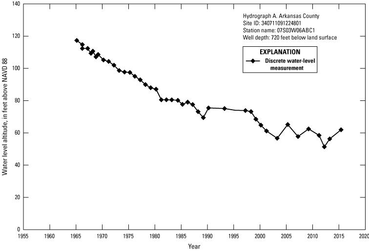
Hydrograph A, Arkansas County.
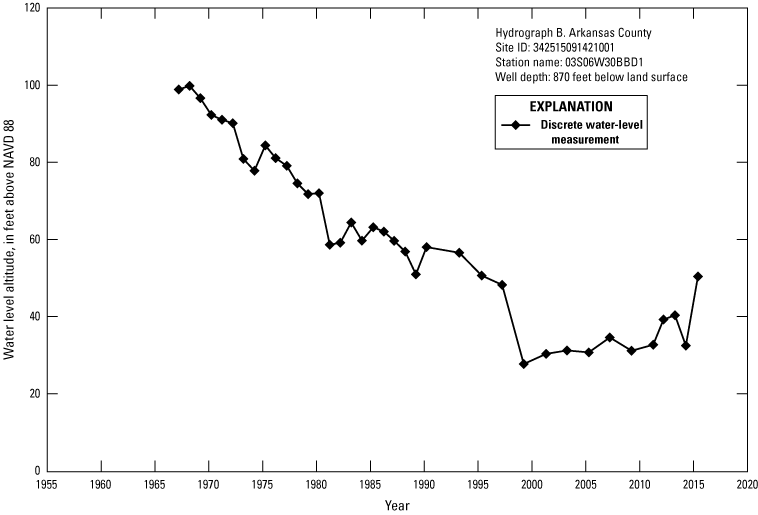
Hydrograph B, Arkansas County.
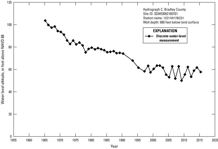
Hydrograph C, Bradley County.
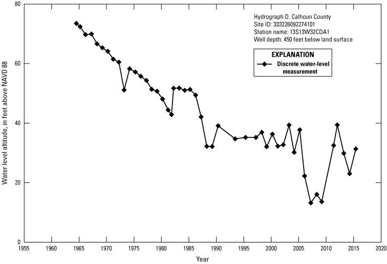
Hydrograph D, Calhoun County.
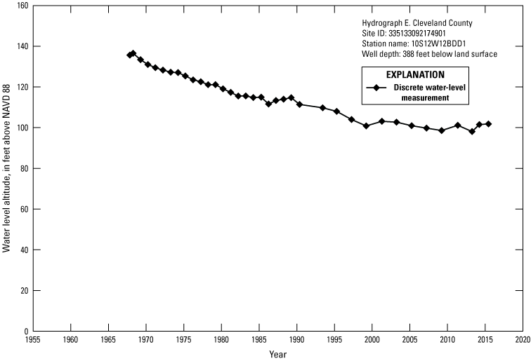
Hydrograph E, Cleveland County.
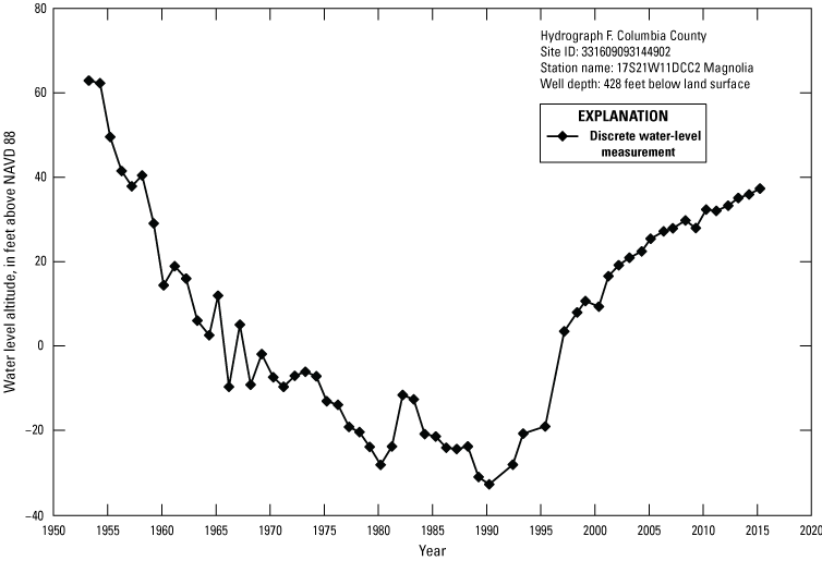
Hydrograph F, Columbia County.
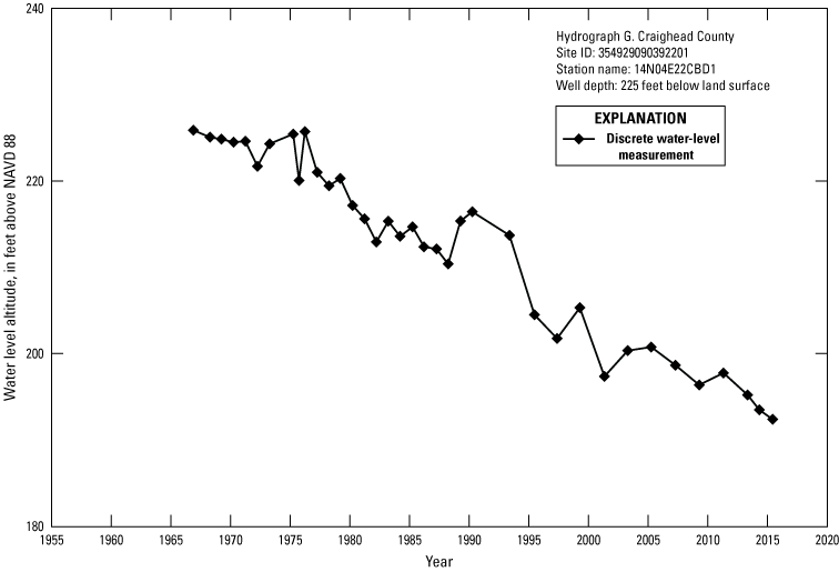
Hydrograph G, Craighead County.
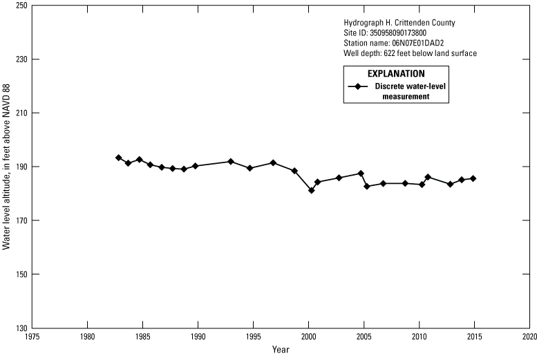
Hydrograph H, Crittenden County.
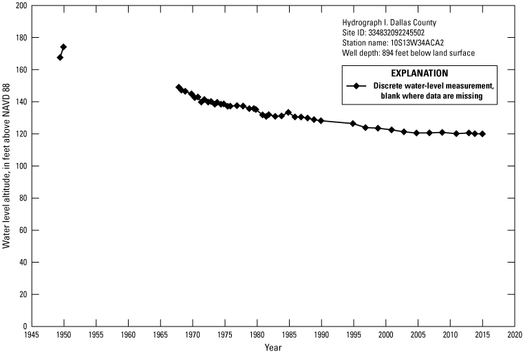
Hydrograph I, Dallas County.
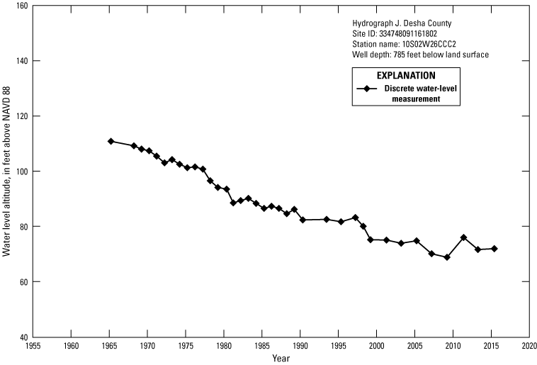
Hydrograph J, Desha County.
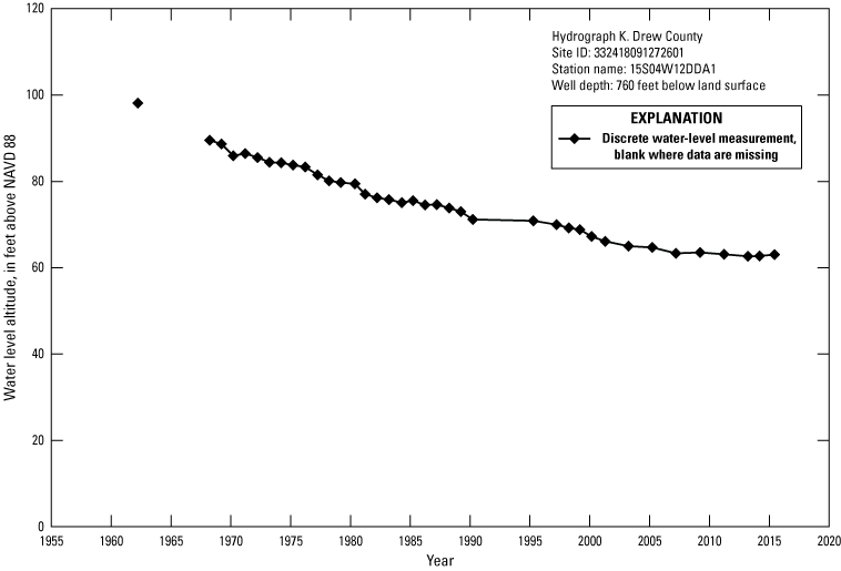
Hydrograph K, Drew County.
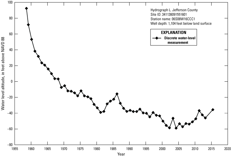
Hydrograph L, Jefferson County.
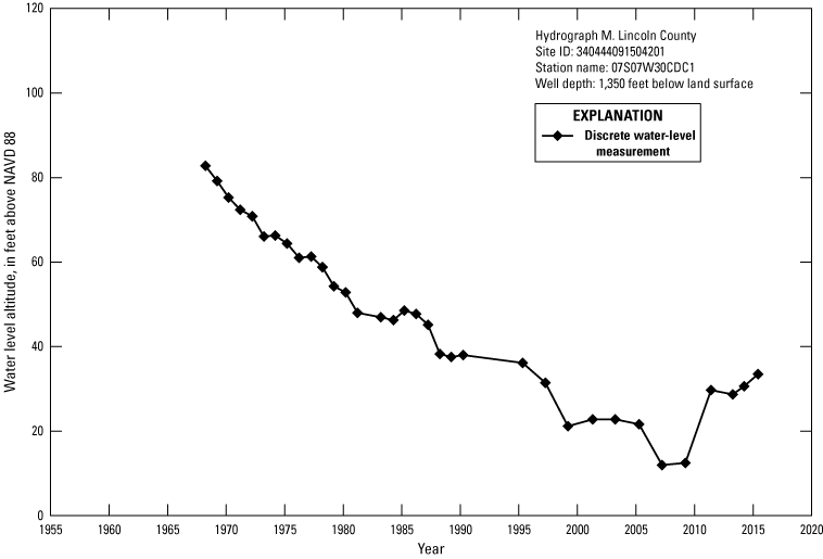
Hydrograph M, Lincoln County.
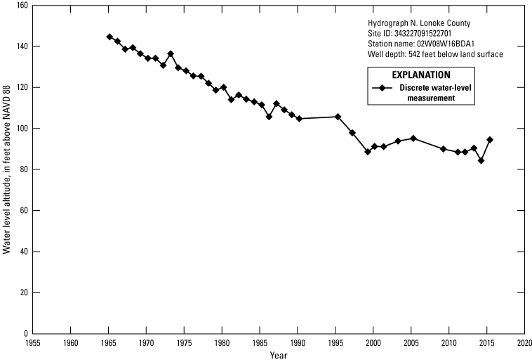
Hydrograph N, Lonoke County.
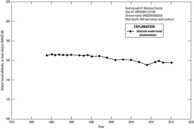
Hydrograph O, Monroe County.
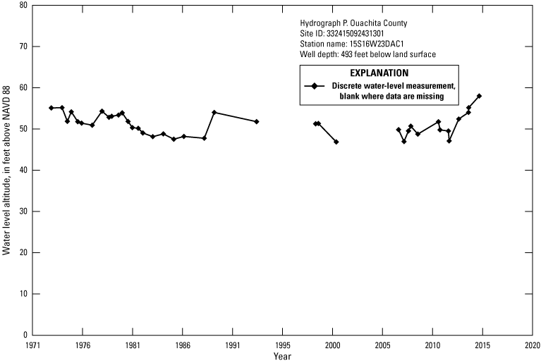
Hydrograph P, Ouachita County.
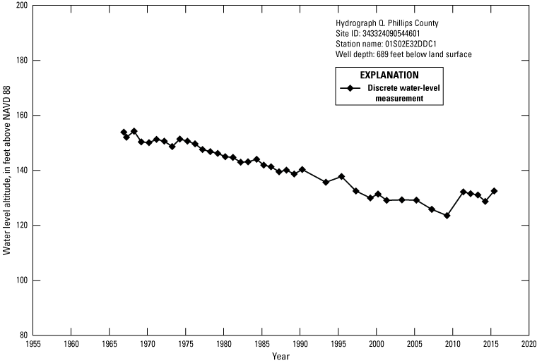
Hydrograph Q, Phillips County.
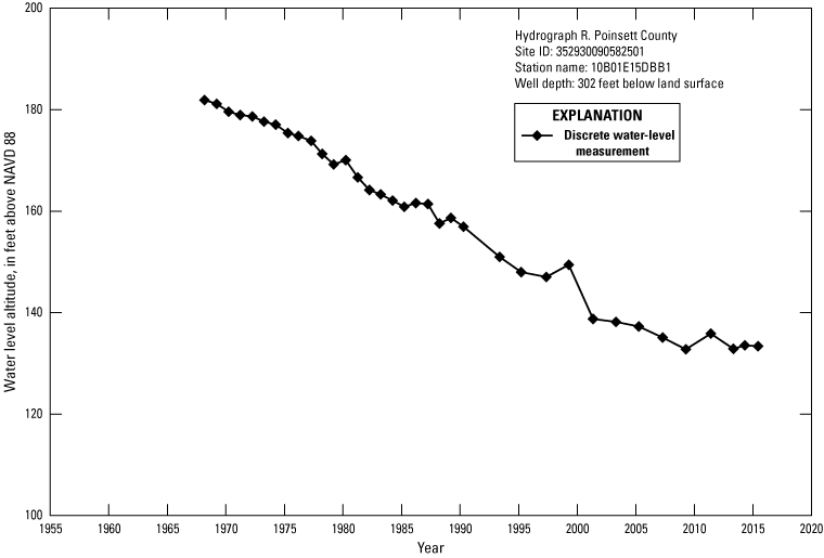
Hydrograph R, Poinsett County.
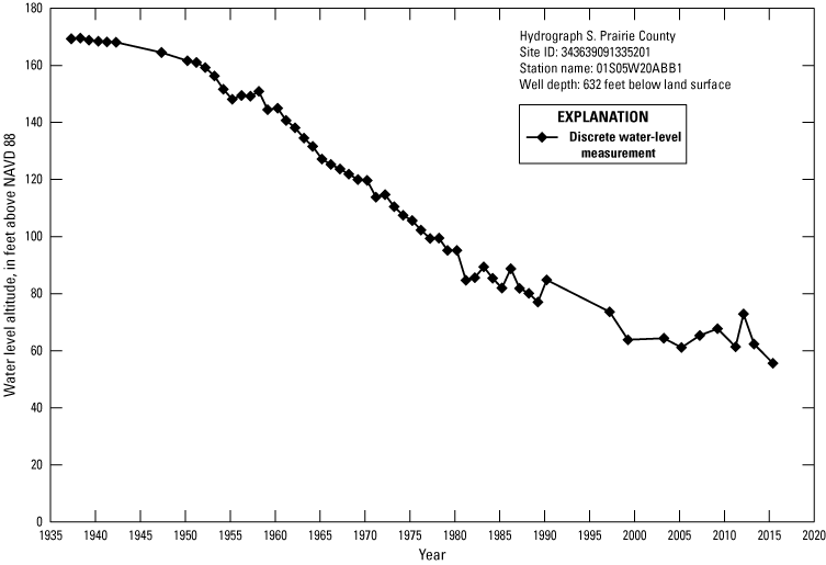
Hydrograph S, Prairie County.
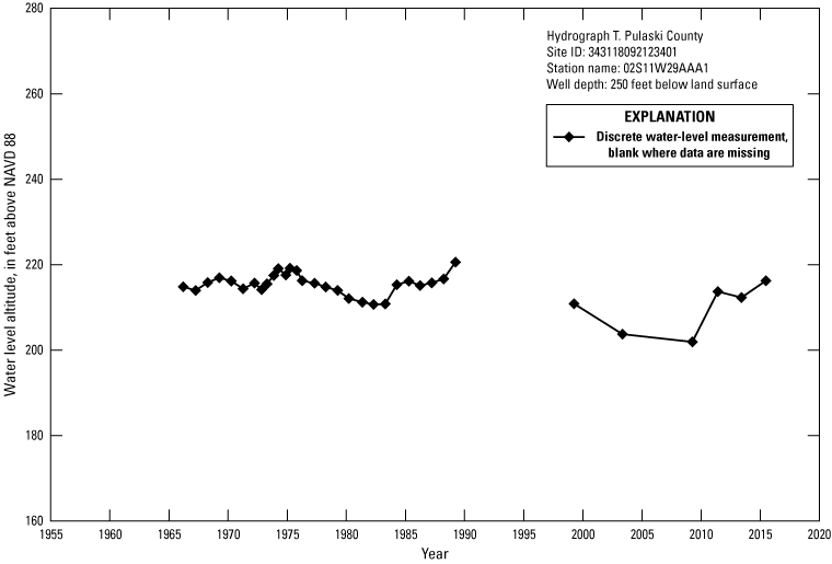
Hydrograph T, Pulaski County.
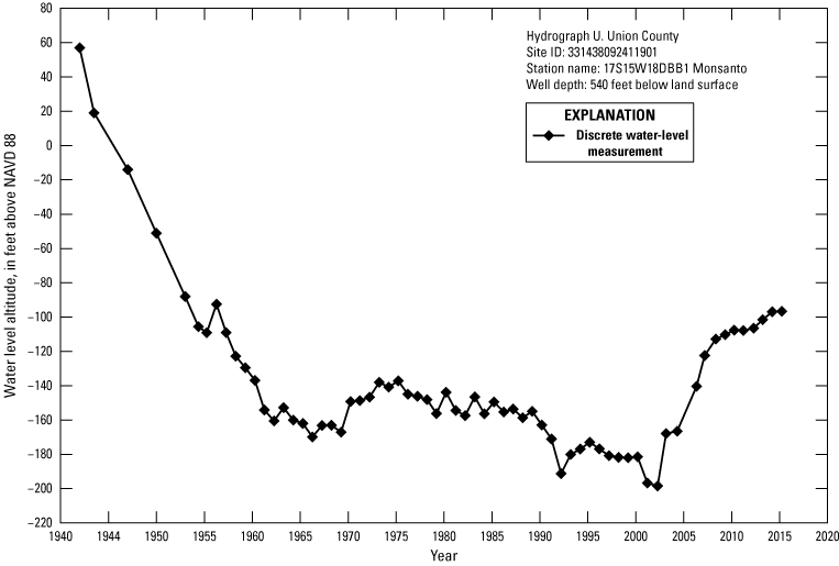
Hydrograph U, Union County.
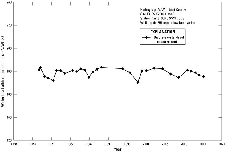
Hydrograph V, Woodruff County.
Appendix 4. Wells and Differences in Water-Levels From 2011 To 2013 in the Sparta-Memphis Aquifer in Arkansas
Appendix 5. Wells and Differences in Water-Levels From 2013 To 2015 in the Sparta-Memphis Aquifer in Arkansas
Conversion Factors
Datum
Vertical coordinate information is referenced to the North American Vertical Datum of 1988 (NAVD 88).
Horizontal coordinate information is referenced to the North American Datum of 1983 (NAD 83).
Altitude, as used in this report, refers to distance above the vertical datum.
Supplemental Information
Specific conductance is given in microsiemens per centimeter at 25 degrees Celsius (µS/cm at 25 °C).
Concentrations of chemical constituents in water are given in milligrams per liter (mg/L).
Abbreviations
ADA–NRD
Arkansas Department of Agriculture-Natural Resources Division
Br
bromide
CGWA
critical groundwater area
Cl
chloride
MRVA
Mississippi River Valley alluvial
PDSI
Palmer Drought Severity Index
QC
quality control
ROS
regression on order statistics
UCWCB
Union County Water Conservation Board
USGS
U.S. Geological Survey
For more information about this publication, contact
Director, Lower Mississippi-Gulf Water Science Center
U.S. Geological Survey
640 Grassmere Park, Suite 100
Nashville, TN 37211
For additional information, visit
https://www.usgs.gov/centers/lmg-water/
Publishing support provided by
Lafayette Publishing Service Center
Disclaimers
Any use of trade, firm, or product names is for descriptive purposes only and does not imply endorsement by the U.S. Government.
Although this information product, for the most part, is in the public domain, it also may contain copyrighted materials as noted in the text. Permission to reproduce copyrighted items must be secured from the copyright owner.
Suggested Citation
Nottmeier, A.M., Knierim, K.J., and Hays, P.D., 2023, Potentiometric surfaces (2013, 2015), groundwater quality (2010–15), and water-level changes (2011–13, 2013–15) in the Sparta-Memphis aquifer in Arkansas: U.S. Geological Survey Scientific Investigations Report 2023–5103, 47 p., https://doi.org/10.3133/sir20235103.
ISSN: 2328-0328 (online)
Study Area
| Publication type | Report |
|---|---|
| Publication Subtype | USGS Numbered Series |
| Title | Potentiometric surfaces (2013, 2015), groundwater quality (2010–15), and water-level changes (2011–13, 2013–15) in the Sparta-Memphis aquifer in Arkansas |
| Series title | Scientific Investigations Report |
| Series number | 2023-5103 |
| DOI | 10.3133/sir20235103 |
| Publication Date | September 28, 2023 |
| Year Published | 2023 |
| Language | English |
| Publisher | U.S. Geological Survey |
| Publisher location | Reston, VA |
| Contributing office(s) | Lower Mississippi-Gulf Water Science Center |
| Description | Report: viii, 47 p.; 2 Data Releases; 4 Plates: 42.00 × 28.00 inches or smaller; 5 Appendixes |
| Country | United States |
| State | Arkansas |
| Other Geospatial | Sparta-Memphis aquifer |
| Online Only (Y/N) | Y |