

Comparison of Hydrologic Data and Water Budgets Between 2003–08 and 2018–23 for the Eastern Part of the Arbuckle-Simpson Aquifer, South-Central Oklahoma
Links
- Document: Report (10.2 MB pdf) , HTML , XML
- Data Release: USGS Data Release - Soil-Water-Balance model and data for Phase 1 (2003–08) and Phase 2 (2018–23) hydrologic and water-budget analyses of the eastern part of the Arbuckle-Simpson aquifer, south-central Oklahoma, 2019–22
- NGMDB Index Page: National Geologic Map Database Index Page (html)
- Download citation as: RIS | Dublin Core
Acknowledgments
This study of the hydrology of the eastern part of the Arbuckle-Simpson aquifer was possible through cooperation with the Oklahoma Water Resources Board of the State of Oklahoma and The Oka’ Institute at East Central University. Additional collaborating partners were the U.S. Fish and Wildlife Service; the National Park Service; the U.S. Environmental Protection Agency, Robert S. Kerr Environmental Research Center; The Chickasaw Nation; The Choctaw Nation of Oklahoma; and Vulcan Materials Company.
The authors would like to thank the Blue River Foundation of Oklahoma for providing input, ideas, information, and time to make this project a success. The authors also thank the many landowners who granted access for collecting data. This report and study would not have been possible without their assistance.
The authors would also like to thank the U.S. Geological Survey staff who have dedicated their time to the success of this project: Jason Lewis, Rick Hanlon, Kevin Smith, Levi Close, Nicholas Pierson, Kyle Cothren, Carol Becker, Stephen Bradford, Steven Smith, Ian Rogers, MaryKate Higginbotham, Natalie Gillard, Cory Russell, Amy Morris, and Nicole Gammill.
Abstract
The Arbuckle-Simpson aquifer is divided spatially into three parts (eastern, central, and western). The largest groundwater withdrawals are from the eastern part of the Arbuckle-Simpson aquifer, which provides water to approximately 39,000 people in Ada and Sulphur, Oklahoma, and surrounding areas. The Arbuckle-Simpson aquifer, including the eastern part, is designated a sole source aquifer for its service area. Based primarily on data collected between 2003 and 2008, a series of comprehensive hydrologic studies of the Arbuckle-Simpson aquifer was published to provide the information necessary to perform groundwater-flow model simulations so that the Oklahoma Water Resources Board could determine how much water could be withdrawn from the aquifer while maintaining flow to springs and streams. As part of the Phase 1 studies, an aquifer water budget was developed from a numerical model for the period 2003–08. For this report, Phase 1 refers to the 2003–08 data collection period, although for some of the analyses, data collected prior to 2003 were used to inform model development work. Allocation of water from this aquifer was then established by the Oklahoma Water Resources Board in 2013. Additional well-spacing rules were also established by the Oklahoma Water Resources Board for sensitive sole source groundwater basins. To determine how the water budget for the eastern part of the Arbuckle-Simpson aquifer has changed over time, recently collected hydrologic data (2018–23) were compared to data collected during 2003–08. The analysis of changes in the aquifer water budget from 2003–08 to 2018–23 could help resource managers better understand changes in the overall balance of water in storage and the potential effects on streamflow, changes in groundwater levels, and the effects of different water uses in the aquifer area on available water in the eastern part of the Arbuckle-Simpson aquifer and streams overlying the eastern part of the Arbuckle-Simpson aquifer.
Introduction
Based primarily on data collected between 2003 and 2008, a series of comprehensive hydrologic studies of the Arbuckle-Simpson aquifer in south-central Oklahoma was conducted between 2003 and 2011. For this report, “Phase 1” refers to an initial 2003–08 data collection period, although for some analyses, data collected prior to 2003 were used to inform model development. Results from Phase 1 provided information necessary to perform groundwater-flow model simulations that, in addition to characterizing groundwater resources in the study area, helped inform the Oklahoma Water Resources Board (OWRB) in their decisions regarding how much water could be withdrawn from the aquifer while maintaining flow to springs and streams. The rocks that contain the karstic Arbuckle-Simpson aquifer consist primarily of uplifted carbonates exposed at the surface across an area of approximately 520 square miles (mi2) (332,800 acres) in Carter, Coal, Johnston, Murray, and Pontotoc Counties (Christenson and others, 2011). In addition to being uplifted, the rocks that contain the Arbuckle-Simpson aquifer are characterized by large fault displacements and folded structures. The Arbuckle-Simpson aquifer is divided spatially into three parts (eastern, central, and western). Christenson and others (2011, p. 4) noted that most groundwater withdrawals are from the eastern part of the Arbuckle-Simpson aquifer, which among other uses, provides water to Ada and Sulphur, Okla., and surrounding areas. The largest streams and springs (by flow volume) also emanate from the eastern part of the Arbuckle-Simpson aquifer. The U.S. Environmental Protection Agency (EPA) designated the Arbuckle-Simpson aquifer, including the eastern part of the Arbuckle-Simpson aquifer, as a “sole source aquifer” in 1989 (EPA, 1989). The EPA defines a sole source aquifer as one where “the aquifer supplies at least 50 percent of the drinking water for its service area” and “there are no reasonably available alternative drinking water sources should the aquifer become contaminated” (EPA, 2024a).
The OWRB manages the use of groundwater and surface-water resources under separate appropriation doctrines, according to Oklahoma water law. Surface water is considered to be publicly owned and subject to appropriation by the OWRB (Oklahoma State Legislature, 2023a). Conversely, groundwater is considered a private property right that belongs to the overlying surface owner, but permits from the OWRB are required for most uses of groundwater, except for most domestic uses (Oklahoma State Legislature, 2023b). In response to concerns about potential transfers of groundwater from the Arbuckle-Simpson aquifer to central Oklahoma, the Oklahoma Senate passed Senate Bill 288 (2003), which imposed a moratorium on the issuance of any temporary groundwater permit for municipal or public water-supply use outside of any county that overlies a “sensitive sole source groundwater basin” until the OWRB completes a hydrologic study and approves a maximum annual yield (the maximum amount of water that can be withdrawn from a specific groundwater basin in any year). This moratorium and hydrologic study requirement were implemented to help ensure that any permit for the removal of water from the groundwater basin will not reduce the natural flow of water from springs or streams emanating from the basin (OWRB, 2003).
As a result of Senate Bill 288, comprehensive hydrologic studies of the Arbuckle-Simpson aquifer were conducted between 2003 and 2011 to obtain the data and information necessary to perform groundwater-flow model simulations. The results of groundwater-flow simulations help to inform the OWRB’s decisions as they work to determine how much water could be withdrawn from the aquifer while maintaining flow to springs and streams (Seilheimer and Fisher, 2008; Christenson and others, 2009, 2011; Faith and others, 2010). Springs are outflows from the groundwater aquifers; changes in springflow over time across an aquifer could be an indicator of changes in aquifer water storage amounts. The OWRB established a maximum annual yield (MAY) in 2013 for the Arbuckle-Simpson aquifer based primarily on simulated effects of groundwater withdrawals on springflows and base flows into streams (OWRB, 2023). Maximum annual yield is a determination by the Board (OWRB) of the total amount of fresh groundwater that can be produced from each basin or subbasin allowing a minimum twenty (20) year life of such basin or subbasin (Oklahoma State Legislature, 2023b). The MAY was set for the entire extent of the Arbuckle-Simpson aquifer (not just for the eastern part of the Arbuckle-Simpson aquifer) to 78,404 acre-feet over the total land area of 392,019 acres, with the resulting equal-proportionate share determined to be 0.20 acre-foot per acre per year (OWRB, 2023). The equal-proportionate share is the maximum annual yield of water from a groundwater basin or subbasin which shall be allocated to each acre of land overlying such basin or subbasin (Oklahoma State Legislature, 2023b).
Since completion of hydrologic studies between 2003 and 2011, the OWRB established rules for sensitive sole source aquifers (Oklahoma State Legislature, 2023c). In addition to the general rules for the taking and use of groundwater in an aquifer with a determined maximum annual yield, the OWRB must also find that the proposed use of groundwater is not likely to degrade or interfere with springs or streams emanating in whole or in part from water originating from the sensitive-sole-source groundwater basin before it may approve the application and issue the appropriate permit. Well-spacing rules for sensitive sole source groundwater basins were established to help determine if taking and use of groundwater would interfere with springs or streams emanating from the aquifer. These rules are “(1) no new or proposed well shall be drilled and completed within 1,320 feet of a spring that flows 50 gallons per minute or more, emanates from the groundwater basin, and is identified in table 1–1 in appendix 1 (modified from Appendix D of Oklahoma State Legislature, 2023c); (2) no new or proposed well shall be drilled and completed within 2 miles of a spring that flows 500 gallons per minute or more, emanates from the groundwater basin and is identified in table 1–1 in appendix 1, unless the Board first determines that the total amount of groundwater authorized to be used from all wells within that radius is no more than 1,600 acre-feet per year; (3) no new or proposed well shall be drilled and completed within 1 mile of a stream segment considered to be perennial in the U.S. Geological Survey's (USGS’s) National Hydrography Dataset (USGS, 2023) and with a base flow of more than 500 gallons per minute that emanates from the groundwater basin” (Oklahoma State Legislature, 2023c).
This report describes the results of a study done by the USGS, in cooperation with the OWRB and the Oka’ Institute, to document recently collected (2018–23) hydrologic data and assess water-budget changes for the area containing the eastern part of the Arbuckle-Simpson aquifer. The 2018–23 hydrologic data were collected as part of a Phase 2 study and were compared to hydrologic data collected during 2003–08 as part of a series of Phase 1 studies; data from Phase 1 are available in Christenson and others (2011). As part of the Phase 1 studies, an aquifer water budget was developed from a numerical model for the period 2003–08. The analysis of changes in the aquifer water budget from 2003–08 to 2018–23 could help resource managers better understand (1) changes in the overall balance of water in storage and potential effects on streamflow, (2) changes in groundwater levels, and (3) the effects of different water uses in the aquifer area on available water in both the eastern part of the Arbuckle-Simpson aquifer and streams overlying the eastern part of the Arbuckle-Simpson aquifer.
Study Area
The largest groundwater withdrawals are from the eastern part of the Arbuckle-Simpson aquifer, which provides water to approximately 39,000 people in Ada and Sulphur, Oklahoma, and surrounding areas (OWRB, 2009). The eastern part of the Arbuckle-Simpson aquifer covers approximately 390 mi2 (249,600 acres) and is the largest of the three parts of the Arbuckle-Simpson aquifer by area and aquifer volume (Christenson and others, 2011). Each part of the Arbuckle-Simpson aquifer is associated with a different predominant structural geological feature: the Hunton Anticline (eastern part of the Arbuckle-Simpson aquifer), the Tishomingo Anticline (central part of the Arbuckle-Simpson aquifer), and the Arbuckle Anticline (western part of the Arbuckle-Simpson aquifer) (Christenson and others, 2011). The hydrologic study and groundwater-flow model in Christenson and others (2011) were focused on the eastern part of the Arbuckle-Simpson aquifer; the eastern part of the Arbuckle-Simpson aquifer is also the focus of this report. Christenson and others (2011, p. 14) noted that the eastern part of the Arbuckle-Simpson aquifer “is dominated by the Hunton anticline, but also includes other structural features, including the Belton and Clarita anticlines, the Sulphur syncline, and the Lawrence uplift.”
Aquifer recharge refers to the process by which water enters a given aquifer and becomes part of the groundwater system (Freeze and Cherry, 1979). Direct recharge from precipitation is the primary source of groundwater in the Arbuckle-Simpson aquifer; little to no inflow of groundwater comes from surrounding aquifers. Groundwater discharge from the aquifer predominantly contributes to streams and springs, including Blue River, Pennington Creek, Mill Creek, and Delaware Creek, which originate as outflows from the aquifer, as well as numerous smaller streams (fig. 1). Groundwater discharge typically maintains base flow in streams overlying the aquifer (although this can change seasonally because of reductions of storage in the aquifer and reduced recharge to the aquifer during dry periods when there is less precipitation). Blue River, which drains a large extent of the eastern part of the Arbuckle-Simpson aquifer, is the largest stream that originates in the study area. Many springs, including Byrds Mill Spring, the primary water supply for the City of Ada, also discharge from the aquifer. During Phase 1, the discharge from Byrds Mill Spring was monitored by USGS streamgage 07334200 Byrds Mill Spring near Fittstown, Okla. (hereinafter referred to as the “Byrds Mill Spring gage” [table 1–1; fig. 2]).
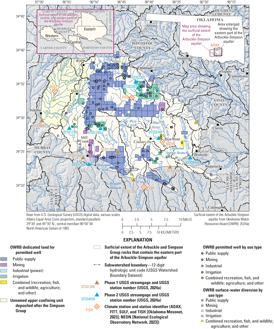
Map of study area showing the eastern part of the Arbuckle-Simpson aquifer, U.S. Geological Survey streamgages where streamflow data were collected for the Phase 1 (2003–08) and Phase 2 (2018–23) studies, climate stations where precipitation data were collected, and surface-water diversions and permitted wells, south-central Oklahoma, 2003–23.
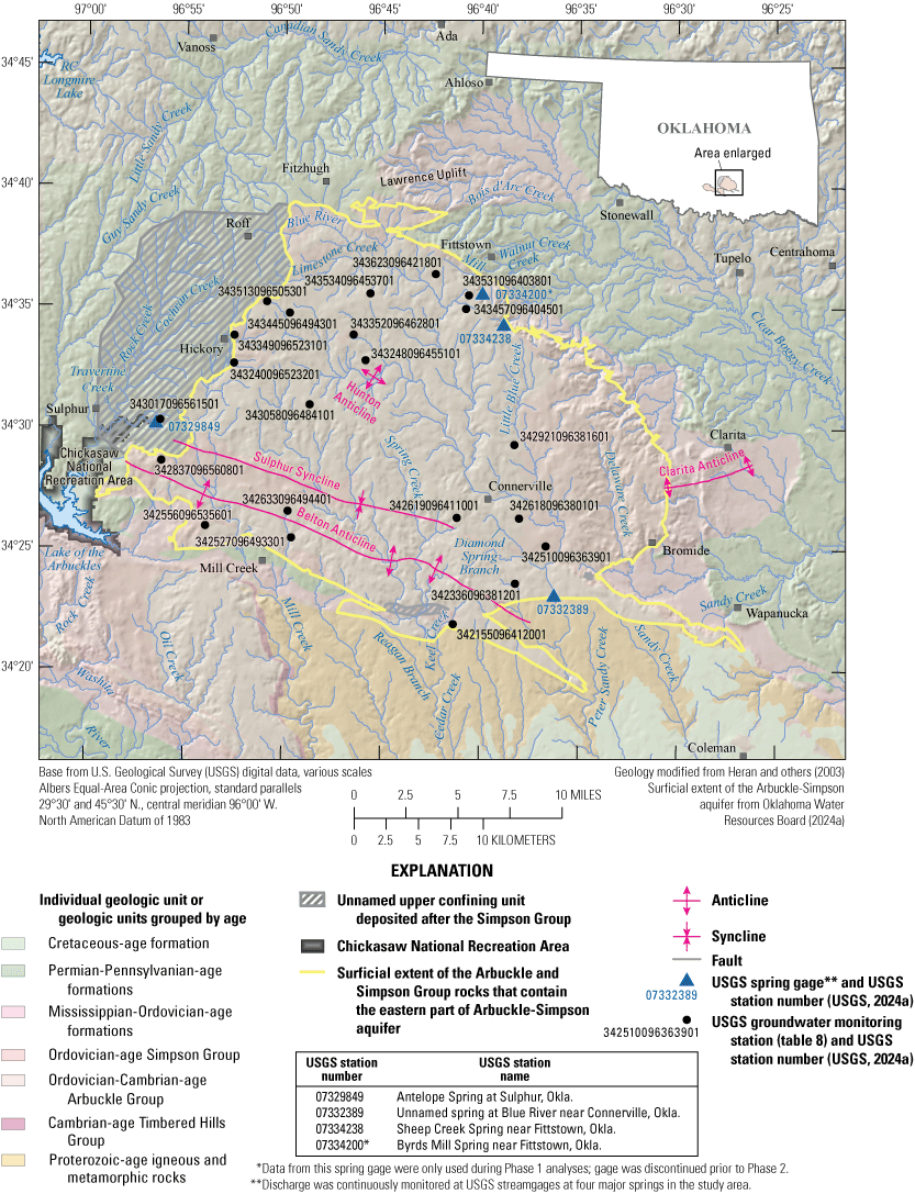
Geologic units exposed at the surface in the study area for the eastern part of the Arbuckle-Simpson aquifer, with locations of U.S. Geological Survey (USGS) groundwater monitoring stations where data were collected for the Phase 2 (2018–23) study and USGS spring gages where spring discharges were measured, south-central Oklahoma.
Purpose and Scope
The purpose of this report is to compare recent hydrologic data collected primarily during 2018–23 as part of a “Phase 2” study to historical hydrologic data collected primarily during 2003–08 and published in Christenson and others (2011) as part of an initial “Phase 1” study to determine how the water budget for the area overlying the eastern part of the Arbuckle-Simpson aquifer has changed. The analysis of changes in the aquifer water budget from 2003–08 to 2018–23 could help resource managers better understand changes in the overall balance of water in storage and potential effects to streamflow, changes in groundwater levels, and the effects of different water uses in the aquifer area on available water in both the eastern part of the Arbuckle-Simpson aquifer and streams overlying the eastern part of the Arbuckle-Simpson aquifer. The organization and wording of this report is largely based on that of Christenson and others (2011).
Geology and Hydrogeologic Units
The rocks that compose the Arbuckle-Simpson aquifer are exposed at the surface in an area of 520 mi2 of south-central Oklahoma, formally known as the Arbuckle Mountains. The topographic relief of these “mountains” is on the order of hundreds of feet, and their appearance is that of rolling hills to the west and an elevated plain to the east (Christenson and others, 2011). The Arbuckle Mountains are composed of Proterozoic- and Cambrian-aged igneous and metamorphic rocks overlain by sedimentary rocks that are Cambrian to Late Pennsylvanian in age (Christenson and others, 2011). The geology of the Arbuckle Mountains is characterized by both macro- and meso-scale deformations, consisting of folded structures, large fault displacements, uplifts, and karstic features developing in their carbonate sedimentary rocks (Fairchild and others, 1990). Sinkholes, caves, springs, and other characteristic karst features are present throughout the Arbuckle Mountains (Christenson and others, 2011). Because all these features affect the flow and availability of groundwater in the study area, the geologic framework of the Arbuckle Mountains is considered when assessing groundwater in the Arbuckle-Simpson aquifer.
Geologic History
The geologic history of the Arbuckle Mountains encompasses more than a billion years, from Proterozoic igneous and metamorphic rocks to Quaternary alluvial deposits. There are four main phases of geologic history, including tectonics and sedimentation, that formed and shaped the Arbuckle Mountains of today: (1) an initial splitting apart of tectonic plates (rifting) during the Early and Middle Cambrian Epochs, (2) deposition and subsidence during the Late Cambrian Epoch through the Mississippian Subperiod, (3) uplift and deformation during the Pennsylvanian Subperiod, and (4) erosion and post-Pennsylvanian Subperiod tilting (Johnson, 1991). Before the first phase of rifting, during the Proterozoic Eon, the study area was underlain primarily by granites and gneisses. About 1.3 billion years ago, during the Proterozoic Eon, igneous dikes were intruded into the surrounding rock, which was the first evidence of crustal weakness that would later alter the geology of the area.
In the Early and Middle Cambrian Epochs, the first phase of crustal deformation occurred, with rifting that caused the development of major normal faults along the margins and more igneous activity. As these igneous rocks cooled in the rift zone, the land surface began to subside, creating a trough that would subsequently be filled with sedimentary rocks.
The Late Cambrian Epoch through the Mississippian Subperiod is marked by the second main phase of geologic history in the region. During this time, shallow seas covered much of the midcontinent of what is now North America, which caused deposition of carbonate sediments that would later become the Arbuckle Group that was deposited during the Late Cambrian Epoch through the Early Ordovician Epoch. Some of these sediments were deposited in the sedimentary trough, which is commonly referred to today as the Southern Oklahoma Aulacogen (Johnson and others, 1989; Chase and others, 2022). Sedimentary rocks that formed in the Southern Oklahoma Aulacogen are much thicker than the surrounding rock, with more than 17,000 feet (ft) of rock accumulation, relative to the surrounding continental shelf, which accumulated about 6,500 ft of rock during the same time period (Ham, 1973). At the end of the Early Ordovician Epoch the sea level decreased enough to expose these carbonate sediments to meteoric waters, resulting in the dolotomization of some rocks in the Arbuckle Group (Lynch and Al-Shaieb, 1991; Denison, 1997). Dolomitization is a process where the carbonate mineral dolomite is formed when magnesium ions replace calcium ions in calcite. This second phase of geologic history also saw the deposition of the Simpson Group of Middle to Late Ordovician age on top of the rocks of the Arbuckle Group. The Simpson Group is composed of marine-shelf carbonates, shales, and quartz sandstones, indicating a shallow-sea depositional environment (Johnson, 1991).
The third phase of geologic history in the Arbuckle Mountains began in the Early Pennsylvanian Epoch and was marked by uplift and deformation, including the formation of the Hunton Anticline in the study area. The Late Pennsylvanian Epoch brought intense mountain building along the margins of the Southern Oklahoma Aulacogen, which resulted in tight folding and high angle thrust faulting of these rocks (Christenson and others, 2011). This mountain building event is thought to have been caused by a major plate collision between the North American plate and Gondwana or another smaller plate during the Late Pennsylvanian Epoch (Perry, 1989).
Finally, the fourth phase of geologic history in the study area is characterized by additional deposition and erosion. After the Late Pennsylvanian Epoch mountain-building event, sediment deposits of Late Pennsylvanian age covered the Arbuckle Mountains. Red beds and evaporites of Permian age were deposited in basins, followed by shallow-sea sand and carbonate deposits of Cretaceous age (Johnson and others, 1989). These shallow seas also caused erosion of the Arbuckle Mountains, which were further flattened by fluvial erosion during the Cretaceous Period (Donovan, 1991). Further erosion and tilting in the study area was due to the uplift of the Rocky Mountains hundreds of miles west of the Arbuckle Mountains during the Laramide orogeny (English and Johnston, 2004). Alluvial and terrace sedimentation of Quaternary age deposited along streams and rivers round out this period of deposition and erosion in the study area (Johnson and others, 1989). A more complete geologic history of the Arbuckle Mountains was detailed by Christenson and others (2011).
Structural Geology
The geologic units that contain the eastern part of the Arbuckle-Simpson aquifer, which is the focus of this study, are shaped primarily by the Hunton Anticline, but include other structural features, including the Belton and Clarita Anticlines, the Sulphur Syncline, and the Lawrence Uplift (fig. 2). The Hunton Anticline is a broad anticlinal fold that exposed the Early Ordovician-age West Spring Creek and Kindblade Formations of the Arbuckle Group to the surface in the central part of the eastern part of the Arbuckle-Simpson aquifer (Johnson, 1990). The northwestern arm of the Hunton Anticline dips gently (less than 20 degrees; Christenson and others, 2011) westward, while the southeastern arm dips gently to the east. The Hunton Anticline is bounded by the Lawrence Uplift to the north, the Franks Fault Zone and the Clarita Fault to the northeast/east, and the Sulphur Fault Zone to the south (Christenson and others, 2011). The Sulphur Fault Zone consists of major northwest-southeast-trending faults, which were first displaced during the formation of basement rocks and were reactivated multiple times during Paleozoic Era rifting and orogeny (Harlton, 1966; Denison, 1995). The Sulphur Fault Zone roughly coincides with the northern edge of the Sulphur Syncline, which is bounded to the south by the South Sulphur Fault. Rocks from the Simpson Group were folded to form the Sulphur Syncline, which terminates to the southeast of the study area in the east and at approximately the Chickasaw National Recreation Area to the west (fig. 2). Results from a geophysical gravity study suggest that the Sulphur Syncline might be a graben rather than a syncline, but the name remains the same (Cates, 1989; Scheirer and Hosford Scheirer, 2006).
South of the Sulphur Syncline lies the Belton Anticline, which makes up the southern portion of the eastern part of the Arbuckle-Simpson aquifer study area. The Belton Anticline is a northwest-plunging folded fault block that is structurally higher than the Hunton Anticline (Christenson and others, 2011). These structurally high areas have been eroded, which has exposed the Early Ordovician-age Cool Creek and McKenzie Hill Formations of the Arbuckle Group to the surface. The Mill Creek Fault marks the southern boundary of the eastern part of the Arbuckle-Simpson aquifer study area. This fault runs nearly parallel to the Sulphur Fault Zone, with a northwest-southeast trend, and is nearly vertical, based on gravity data collected near the Chickasaw National Recreation Area (Christenson and others, 2011). Several other small faults in a range of orientations mark the subsurface of the study area, further enhancing disjointed and preferential groundwater-flow paths (Fairchild and others, 1990; Riley, 2004; Scheirer and Hosford Scheirer, 2006; Sample, 2008; Kennedy and others, 2009; Halihan and others, 2009a; Smith and others, 2009; Young and others, 2009; Ramachandran and others, 2012). Detailed visualizations of the structural geology of the eastern part of the Arbuckle-Simpson aquifer area, including geologic unit outcroppings, major faults, structural features, and cross sections, can be found in figures 4, 6, and 7 of Christenson and others (2011).
Hydrogeologic Units
The geologic units of the Arbuckle Mountains, which include the units that contain the Arbuckle-Simpson aquifer, are basement rocks (Cambrian rhyolites and Proterozoic granites and gneisses), the Timbered Hills Group of Late Cambrian age, the Arbuckle Group, and the Simpson Group.
The basement rocks of the Arbuckle Mountains were formed in the Ectasian Period of the Mesoproterozoic Era and are the oldest rocks in the study area at 1.35 to 1.4 billion years old (Ham and others, 1964). They consist of igneous and metamorphic rocks and include the Tishomingo Granite, Troy Granite, and unnamed granodiorite and granitic gneiss. In the eastern part of the Arbuckle-Simpson aquifer study area, these basement rocks are only exposed at the surface as the core of the Belton Anticline in the southern part of the study area (Ham and others, 1964; Denison, 1973). These igneous and metamorphic rocks are cut by several Proterozoic- and Cambrian-age dikes and extrusive pyroclastic rocks. No high-yield water wells are completed in these igneous and metamorphic rocks because they are believed to have very low hydraulic conductivity due to their crystalline structure (Christenson and others, 2011). As a result, these basement rocks form a lower confining unit to the eastern part of the Arbuckle-Simpson aquifer with depths ranging from 3,100 to 4,600 ft below land surface (bls) (Campbell and Weber, 2006).
The Arbuckle Group overlies the Timbered Hills Group and consists of Late Cambrian- to Early Ordovician-age carbonate rocks. The Arbuckle Group is approximately 3,000 ft thick in most of the eastern part of the Arbuckle-Simpson aquifer study area but has been eroded away over parts of the Belton Anticline (Christenson and others, 2011). The Arbuckle Group is divided into eight formations, which include the Fort Sill Limestone and Royer Dolomite of Late Cambrian age, the Signal Mountain Formation of Early Ordovocian age, and the Butterly Dolomite, McKenzie Hill Formation, Cool Creek Formation, Kindblade Formation, and West Spring Creek Formation of Early Ordovocian age, from oldest to youngest (fig. 3). Dolostones are the most common type of carbonate rock in the Arbuckle Group in the eastern part of the Arbuckle-Simpson aquifer (Ham, 1945). Numerous unconformities throughout the Arbuckle Group are evidence that the carbonate rocks were exposed to weathering, encouraging the development of karst features. Surface exposures of the Arbuckle Group, as well as cores of the subsurface, show examples of paleokarst features including dissolution in fractures and cavities, vuggy porosity, and collapse breccias. These paleokarst features increase the porosity of rocks in the Arbuckle Group, also increasing their permeability (Lynch and Al-Shaieb, 1991). The Arbuckle Group is the larger (by both area and thickness) of the two lithostratigraphic groups that contain the Arbuckle-Simpson aquifer. The portion of the Arbuckle-Simpson aquifer contained in the Arbuckle Group is also more productive than the portion contained in the Simpson Group (Christenson and others, 2011) because of its intercrystalline porosity and because of the numerous fractures, solution channels, and cavities it contains (Fairchild and others, 1990). Wells completed in the portion of the Arbuckle-Simpson aquifer contained in the Arbuckle Group typically yield 200 to 500 gallons per minute (gal/min), with some deeper wells reported to yield up to 2,500 gal/min (Fairchild and others, 1990; Christenson and others, 2011).
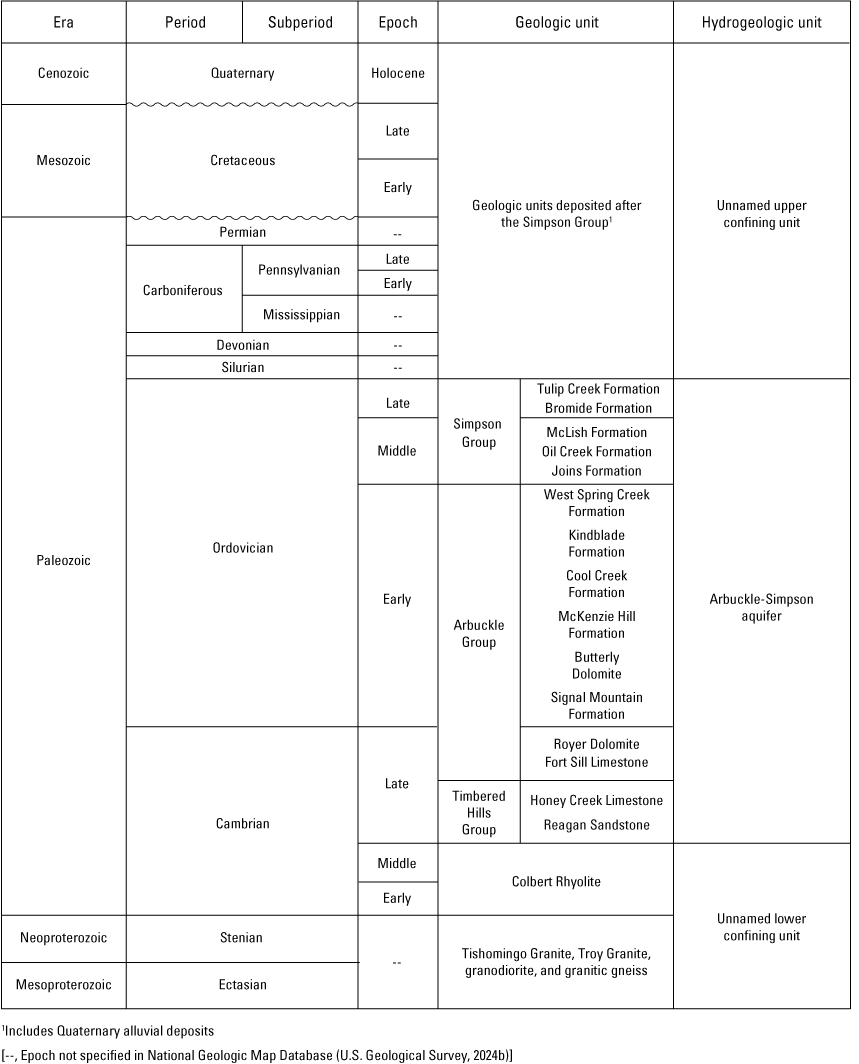
Notable geologic and hydrogeologic units in the eastern part of the Arbuckle-Simpson aquifer. Modified from Christenson and others (2011).
The Simpson Group is the younger of the lithostratigraphic groups contained in the Arbuckle-Simpson aquifer. The Simpson Group is generally less than 1,000 ft thick in the eastern part of the Arbuckle-Simpson aquifer and is exposed at the surface in about one-third of the total aquifer area (145 mi2; Christenson and others, 2011), typically along the edges of major anticlines and other structurally low areas. Erosion over the structurally higher locations in the aquifer has removed the Simpson Group from those areas (Ham, 1973). The largest outcrop of the Simpson Group in the eastern part of the Arbuckle-Simpson aquifer is on the eastern flank of the Hunton Anticline, with another exposure on the Sulphur Syncline.
The Simpson Group was deposited during a time of sea level fluctuations, which resulted in the formation of porous quartzose sandstones interbedded with limestones, dolostones, and greenish-gray shales. The Simpson Group consists of five formations: the Joins, Oil Creek, and McLish Formations of Middle Ordovician age, and the Tulip Creek and Bromide Formations of Late Ordovician age (fig. 3). Because the Joins and Tulip Creek Formations are either very thin or absent in the eastern part of the Arbuckle-Simpson aquifer (Christenson and others, 2011), they will not be discussed further. The most well-developed formations in the eastern part of the Arbuckle-Simpson aquifer are the basal Oil Creek and McLish Formations, which have sandstones with thicknesses of up to 400 and 165 ft, respectively (Ham, 1945; Denison, 1997). These thick beds of uncemented quartz sandstones are mined locally to produce glass, and they store the majority of the water in the part of the eastern part of the Arbuckle-Simpson aquifer contained in the Simpson Group. Wells completed in the eastern part of the Arbuckle-Simpson aquifer contained in the Simpson Group typically yield 100 to 200 gal/min (Fairchild and others, 1990).
Where the top of the eastern part of the Arbuckle-Simpson aquifer is not exposed at the surface, it is confined above by younger rocks of various ages deposited after the Simpson Group (fig. 3). This unnamed upper confining unit confines the eastern part of the Arbuckle-Simpson aquifer on the western edge of the Hunton Anticline, near Sulphur, Okla., and Chickasaw National Recreation Area. This unnamed upper confining unit consists primarily of conglomerate with some sandstone, shale, and minor nodular limestone and lies unconformably over the Arbuckle and Simpson Groups.
Quaternary alluvial deposits are the youngest sediment deposits in the study area. These deposits, consisting of unconsolidated gravel, sand, silt, and clay, are primarily found along larger streams in the study area and are typically very thin and poorly defined. The nature of the Quaternary alluvial deposits is such that they likely would not have the properties of a confining unit; however, these deposits are also not expected to have appreciable hydrologic interaction with the eastern part of the Arbuckle-Simpson aquifer and were, therefore, included in the unnamed upper confining unit for simplicity.
Previous Hydrologic Studies and Phase 1 Study of the Arbuckle-Simpson Aquifer
Hydrologic studies of the Arbuckle-Simpson aquifer were conducted between 2003 and 2011 documenting information that, in addition to characterizing the resources of the study area, helped the OWRB determine how much water could be withdrawn from the aquifer while maintaining flow to springs and streams. These previous hydrologic studies were completed by the USGS in cooperation with OWRB and by other entities working in collaboration with the USGS and OWRB, including the Bureau of Reclamation, Oklahoma State University, and University of Oklahoma (Vieux and Moreno, 2008; Christenson and others, 2009, 2011; Halihan and others, 2009a, b; Puckette, 2009; Puckette and others, 2009; Rahi and Halihan, 2009, 2012; Smith and others, 2009; Tarhule, 2009; Faith and others, 2010). In this report, Phase 1 refers to the study and data published in Christenson and others (2011); as mentioned in the Introduction section, Phase 1 data were primarily collected during 2003–08. The Christenson and others (2011) report includes an aquifer-wide Arbuckle-Simpson study, but the groundwater-flow model was developed for only the eastern part of the Arbuckle-Simpson aquifer (fig. 1). This series of studies is collectively known as the “Arbuckle-Simpson hydrology study.”
The following are objectives of the Arbuckle-Simpson hydrology study.
-
1. Characterize the Arbuckle-Simpson aquifer in terms of geologic setting, aquifer boundaries, hydraulic properties, water levels, groundwater flow, recharge, discharge, and water budget.
-
2. Characterize the area’s surface hydrology, including stream and spring discharge, runoff, base flow, and the relation of surface water to groundwater.
-
3. Construct a digital groundwater/surface-water-flow model of the Arbuckle-Simpson aquifer system for use in evaluating the allocation of water rights and simulating management options.
-
4. Determine the chemical quality of the aquifer and principal streams, identify potential sources of natural contamination, and delineate areas of the aquifer that are most vulnerable to contamination.
-
5. Construct network stream models of the principal stream systems for use in the allocation of water rights.
-
6. Propose water management options, consistent with State water laws, that address water rights issues, the potential impacts of pumping on springs and stream base flows, water quality, and water-supply development.
Hydrologic Data Comparison: Phase 1 to Phase 2
Comparing hydrologic data from Phase 1 to data from Phase 2 will help resource managers better understand changes in streamflow, groundwater levels, and recharge to the aquifer. Different water uses in the aquifer area affect available groundwater storage and base flows in streams overlying the eastern part of the Arbuckle-Simpson aquifer. Although most of the data used in the Phase 1 were from 2003–08, additional data from years prior to 2003 were included in some of the analyses to inform the numerical model. Similarly, most of the data used in Phase 2 were from 2018–23, but additional data from prior years were included in some of the analyses to inform the conceptual water budget. In all instances where data from prior years were included, the nature of the data and the years when the data were collected are explained. The data used in this report are available in the companion USGS data release (Mashburn and others, 2025).
Climate
The bulk of the eastern part of the Arbuckle-Simpson aquifer extends across four counties in southern Oklahoma: Coal, Johnston, Pontotoc, and Murray. These counties are in Oklahoma's south-central climate division, Climate Division 8. Climate Division 8 is characterized by the highest annual mean temperatures and the fourth highest annual mean precipitation values of the nine climate divisions in Oklahoma (Oklahoma Climatological Survey, 2023). Precipitation and temperature data for south-central Oklahoma were analyzed for the years 1895–2022 (fig. 4). Within this period, the minimum temperature recorded was 16.4 degrees Fahrenheit (°F) in February 1899, and the maximum recorded temperature was 104.7 °F in August 2011, with an overall increase in temperature of 0.04 °F per decade during the 1895–2022 period (National Centers for Environmental Information [NCEI], 2023). Annual cumulative precipitation values in south-central Oklahoma increased 0.41 inch per decade during the 1895–2022 period, with a maximum of 70.50 inches reported in 2015 and a minimum of 20.20 inches reported in 1963 (NCEI, 2023). At the time when many of the analyses in this report were completed, precipitation data were only available through 2022. The mean annual precipitation for the 1895–2022 period was 37.97 inches per year (in/yr).
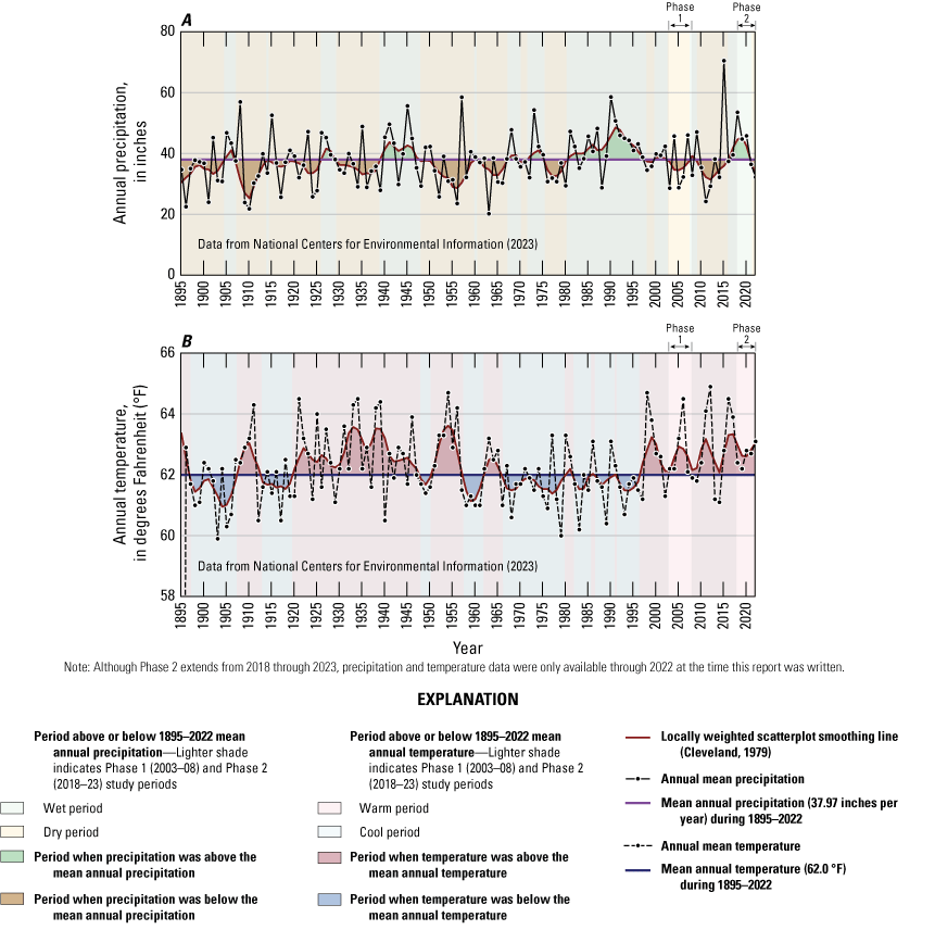
A, Annual mean precipitation with periods of above or below mean annual precipitation and B, annual mean temperature data with periods of above or below the mean annual temperature, south-central Oklahoma, 1895–2022.
Climate division data were also used to compare monthly variation in temperature and precipitation (fig. 5), including comparing mean monthly precipitation and temperature from the entire period of record to the periods of Phase 1 and Phase 2. All three periods of analysis follow similar monthly patterns, with temperature peaking in July–August and precipitation peaking in May–June. Mean monthly precipitation was greater in Phase 2 than in Phase 1 for the months of January, February, March, April, May, August, September, October, and December. Mean monthly temperatures were warmer in Phase 2 than in Phase 1 for the months of May, June, July, August, September, and December.
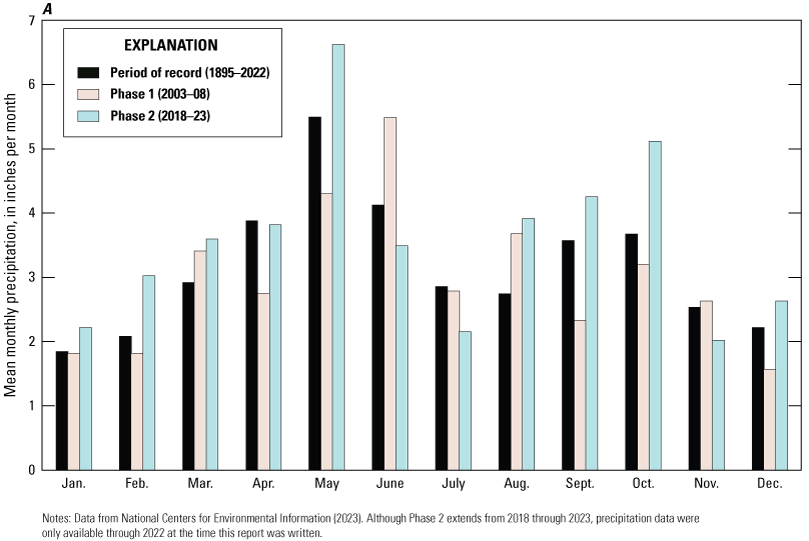
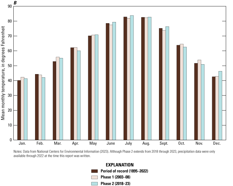
A, Mean monthly precipitation and B, mean monthly temperature for south-central Oklahoma Climate Division 8 during 1895–2022, 2003–08, and 2018–22.
In addition to information for Climate Division 8, data from several individual climate stations in and near the eastern part of the Arbuckle-Simpson aquifer were compiled to further categorize the climate of the region and relate to other data provided within the report. Annual precipitation values were summarized for the Mesonet stations in Ada, Fittstown, Sulphur, and Tishomingo, Okla. (fig. 1; table 1; Oklahoma Mesonet, 2023). Monthly precipitation data at the Blue River site, maintained by the National Science Foundation’s National Ecological Observatory Network (National Ecological Observatory Network [NEON], 2023), were summarized for September 2018–June 2022 (table 2).
Table 1.
Annual precipitation at Mesonet climate stations and the mean precipitation recorded by those Mesonet stations each year (Oklahoma Mesonet, 2023), 1995–2022, south-central Oklahoma.[N/A, data not available]
Ada station (ADAX; fig. 1), Pontotoc County, Okla., latitude 34.798510 decimal degrees (dd), longitude −96.669090 dd.
Fittstown station (FITT; fig. 1), Pontotoc County, Okla., latitude 34.552050 dd, longitude −96.717790 dd.
Tishomingo station (TISH; fig. 1), Johnston County, Okla., latitude 34.332620 dd, longitude −96.678950 dd.
Sulphur station (SULP; fig. 1), Murray County, Okla., latitude 34.566100 dd, longitude −96.950480 dd.
Table 2.
Monthly precipitation recorded by the Blue River NEON station (National Ecological Observatory Network [NEON], 2023), September 2018–June 2022, Johnston County, Oklahoma.[N/A, data not available; dd, decimal degrees]
NEON Blue River station (fig. 1), Johnston County, Okla., 34.444218 decimal degrees (dd), −96.624201 dd.
Streamflow Monitoring
Streamflow data were collected by using a collection of standardized USGS methods described in Sauer and Turnipseed (2010), Turnipseed and Sauer (2010), and Levesque and Oberg (2012). Sauer and Turnipseed (2010) describe the instrumentation and methods used for the acquisition of gage-height data. Turnipseed and Sauer (2010) describe the equipment and procedures used by the USGS for making streamflow measurements. Levesque and Oberg (2012) describe techniques for computing discharge records by using the index velocity method.
Seven new USGS streamgages that monitor discharge were installed on streams flowing across the eastern part of the Arbuckle-Simpson aquifer as a part of Phase 2; in addition, five streamgages in the study area were used to monitor streamflow during Phase 1 and were still operational at the start of Phase 2 (table 3; fig. 1). Discharge readings were recorded at the streamgages in either 15- or 30-minute intervals and transmitted to the USGS National Water Information System (NWIS) database (USGS, 2024a). The time-interval data were averaged at the end of each day and used to report daily mean discharge in cubic feet per second, and the data are all publicly available in NWIS.
Table 3.
Periods of record for U.S. Geological Survey streamgages in and near the eastern part of the Arbuckle-Simpson aquifer, south-central Oklahoma.[USGS, U.S. Geological Survey; OK, Oklahoma; Cr, Creek; 3Mile, Threemile; Blw, below; Del, Delaware; RSVR, reservoir; nr, near. Data are from USGS (2024a). Dates are in year-month-day format. Phase 1 refers to the 2003–08 data collection period; Phase 2 refers to the 2018–23 data collection period]
Threemile Creek is the official name for 3Mile Creek (U.S. Board on Geographic Names, 2024).
In streams that cross the surficial exposure of the rocks containing the eastern part of the Arbuckle-Simpson aquifer, streamflow tends to follow seasonal precipitation patterns. Streamflow is generally highest across all streams in the study area during the spring (March–May) when precipitation rates are higher and evapotranspiration rates are lower compared to the other seasons. Streamflow is lowest in the summer (June–August) and winter (December–February), likely because of lower precipitation rates compared to the spring (April–May) and fall (September–November), as well as higher evapotranspiration rates in the summer. These seasonal differences indicate that higher streamflows are dominated by runoff sources, whereas lower streamflows are dominated by base flow from groundwater sources (groundwater inflows to streams from the eastern part of the Arbuckle-Simpson aquifer).
Other streamgages in the study area include USGS streamgage 07329849 for groundwater sites using township, range, and section information: 01S, Township 01 South; 03E, Range 03 East; 01, Section 01; ABB, Northeast quarter of the Northwest quarter of the Northwest quarter of the section; 1, number designating that this is the first site in the NWIS database with this location information Antelope Spring at Sulphur, Okla. (hereinafter referred to as the “Antelope Spring gage”), USGS streamgage 07332389 unnamed spring at Blue River near Connerville, Okla. (hereinafter referred to as the “unnamed Blue River spring gage”), and USGS streamgage 07334238 Sheep Creek Spring near Fittstown, Okla. (hereinafter referred to as the “Sheep Creek Spring gage”) (fig. 2). The median daily flow at the Antelope Spring gage, USGS streamgage 07329852 Rock Creek at Sulphur, Okla., USGS streamgage 07331200 Mill Creek near Mill Creek, Okla., and USGS streamgage 07331300 Pennington Creek near Reagan, Okla. (hereinafter referred to as “Pennington Creek near Reagan gage”) decreased by 21.9 to 37 percent between Phases 1 and 2. Median daily streamflow at the USGS streamgage 07332390 Blue River near Connerville, Okla. (hereinafter referred to as the “Blue River streamgage”) increased between Phases 1 and 2. The Byrds Mill Spring gage was discontinued prior to Phase 2.
Maximum daily streamflow values increased at most sites that were monitored as a part of the Phase 1 studies, whereas minimum daily streamflow values decreased at every site that was monitored in both Phase 1 (table 4) and Phase 2 (table 5) studies. Compared to smaller precipitation events, the largest (maximum) precipitation events generated more runoff and less recharge to the aquifer during both phases. The reduced minimums in streamflow during Phase 2 are indicative of less recharge and longer dry periods between large precipitation events. Overall, a larger range of streamflow values was observed in Phase 2 than in Phase 1. Water levels in the aquifer were affected by drought conditions, which lasted from 2011 to 2015, followed by a period of heavy precipitation and flooding in 2015 (2015 was the wettest year during the 1895–2011 period; fig. 4A). These climate conditions affected the maximum and minimum discharge values observed in Phase 2 as compared to those of Phase 1.
Table 4.
Summary statistics for streamgages used during Phase 1 for the eastern part of the Arbuckle-Simpson aquifer, south-central Oklahoma.[USGS, U.S. Geological Survey; ft3/s, cubic foot per second. Data are from USGS (2024a). Dates are in year-month-day format]
Table 5.
Changes in daily streamflow between Phase 1 and Phase 2 for the eastern part of the Arbuckle-Simpson aquifer, Oklahoma.[USGS, U.S. Geological Survey; ft3/s, cubic foot per second. Data are from USGS (2024a). Dates are in year-month-day format; N/A, not applicable]
Base Flow
Base-flow separation is the method of separating the base-flow or groundwater component from the runoff component to determine the percentage of each that compose the total streamflow. Base-flow separation methods are based on the assumptions that water discharging an aquifer to a stream is continuous. Over time, changes in the ratio of base flow to total streamflow may indicate changes in groundwater storage or availability. Base-flow separation was completed by using the PART program of the USGS Groundwater Toolbox (Barlow and others, 2015). The PART method uses streamflow partitioning to estimate daily base flow from the streamflow record and is based on the antecedent streamflow recession (Rutledge, 1998; fig. 6). The PART method is used for the analysis of the groundwater-flow system of a basin for which a streamflow-gaging station at the downstream end can be considered the only point of outflow. One assumption of the PART method is that the area of the contributing groundwater-flow system is equal to the drainage area of the streamflow-gaging station for the purpose of expressing flow in units of specific discharge (length per time). To use the PART method, regulation and diversion of flow should be negligible and the drainage-basin area should be less than 500 mi2 (Rutledge, 1998). For this report, negligible regulation for a streamflow-gaging station is defined as having less than 20 percent of the drainage area upstream from a streamflow-gaging station controlled by dams, floodwater-retarding structures, or other human modifications of streamflow. Analysis of hydrographs using PART results in periods of time (annual, monthly, seasonal) with base-flow and runoff portions of streamflow for which base-flow percentages can be calculated. Base-flow separation during Phase 1 and Phase 2 was done by using the PART hydrograph-separation method included in the USGS Groundwater Toolbox (Barlow and others, 2015). For the PART hydrograph-separation computations, the subsurface watershed areas used were from table 8, page 39, in Christenson and others (2011).
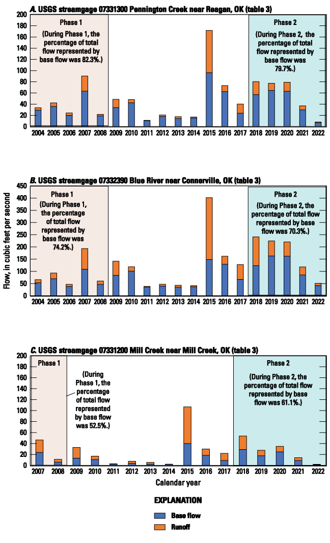
Annual mean base-flow estimates and mean annual base-flow for selected streams crossing the eastern part of the Arbuckle-Simpson aquifer Phase 1 (2003–08) to Phase 2 (2018–23), south-central Oklahoma.
Base-flow separation was completed for the Phase 1 studies for calendar years 2004–08 for the streamflow records collected at the Blue River streamgage and Pennington Creek near Reagan gage, and for calendar years 2007–08 for the streamflow records collected at USGS streamgage 07331200 Mill Creek near Mill Creek, Okla. (hereinafter referred to as the "Mill Creek near Mill Creek gage"). Mean annual base flow was 74.2 percent of the total streamflow measured at the Blue River streamgage (fig. 6). Mean annual base flow computed at the Pennington Creek near Reagan gage was 82.8 percent of the total streamflow measured in Pennington Creek. Mean annual base flow computed at the Mill Creek near Mill Creek gage was 52.5 percent of the total streamflow measured in Mill Creek. The streamflow measured at the Byrds Mill Spring gage was 100 percent base flow because it consisted entirely of groundwater issuing from Byrds Mill Spring with no surface-water component. During 1990–2005, streamflow at the Byrds Mill Spring gage averaged 18.5 cubic feet per second (ft3/s).
Base-flow separation was completed for Phase 2 for calendar years 2018–22 at the Blue River streamgage, the Pennington Creek near Reagan gage, and the Mill Creek near Mill Creek gage. Mean annual base flow at the Blue River streamgage was 70.3 percent of the total streamflow (fig. 6). Mean annual base flow at the Pennington Creek near Reagan gage was 79.7 percent of the total streamflow. Mean annual base flow at the Mill Creek near Mill Creek gage was 61.1 percent of the total streamflow. Base flow increased from Phase 1 to Phase 2 at all three streamgages. However, the base-flow portion of streamflow decreased from Phase 1 to Phase 2 at two of the three streamgages analyzed (fig. 6).
One issue with attempting to compute the base-flow portion of streamflow is the influence of anthropogenic discharges upstream, such as stream augmentation from producing mines (described in the “Consumptive Water Use at Producing Mines” section of this report). These discharges affect streamflows measured and analyses of streamflows for interpretation of groundwater and surface-water interactions and base-flow analyses (fig. 7). The increases in the base-flow portion of streamflow and total streamflow during Phase 2 (fig. 6C) could be related to these upstream discharges.
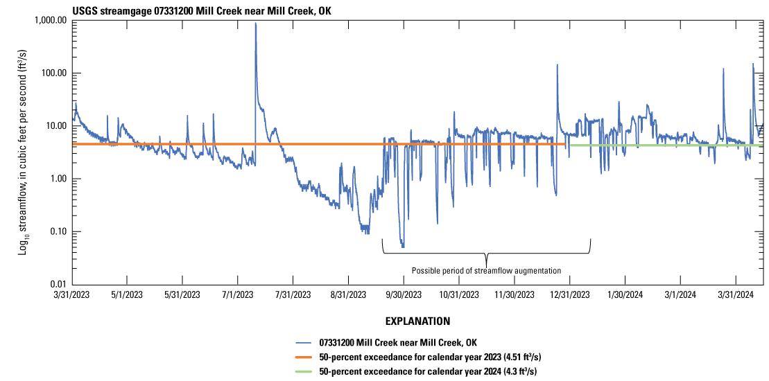
Streamflow before, during, and after augmentation from producing-mine discharges upstream from U.S. Geological Survey streamgage 07331200 Mill Creek near Mill Creek, Oklahoma, March 2023–April 2024.
Net Streamflow Gains and Losses
Net gains and losses in streamflow along stream segments can be quantified by using discrete discharge measurements made during base-flow conditions, commonly referred to as synoptic base-flow (seepage-run) measurements. Locations of these measurements can be mapped to illustrate interactions with the underlying aquifer during base-flow conditions. Discharge was measured at 40 stream locations at USGS stations, including several USGS streamgages, across the land surface overlying the aquifer in each stream main stem and selected tributaries (table 6; figs. 8–9). The relative net gain or loss of groundwater from or to the aquifer for each stream segment between two measurements was calculated (figs. 8–9). To ensure base-flow conditions were being captured, with as little runoff as possible, streamflow discharge was measured during January 24–31, 2022 (fig. 8), and February 28–March 1, 2023 (fig. 9), when evapotranspiration and groundwater withdrawals were considered minimal and after runoff from any precipitation events had dissipated (streamflow hydrographs in and near the study area were analyzed to ensure runoff had dissipated). Fewer sites were measured in 2023 due to lack of access to sites.
Table 6.
Discrete discharge measurements made as part of the 2022 and 2023 seepage runs in and near the study area for the eastern part of the Arbuckle-Simpson aquifer, south-central Oklahoma.[USGS, U.S. Geological Survey; ft3/s, cubic foot per second; blw, below; OK, Oklahoma; nr, near; N, north; E, east; W, west; Rd, road; 3Mile, Threemile; abv, above; Cr, Creek; Rvr, River; CCDC, southwest quarter of the southeast quarter of the southwest quarter of the southwest quarter; Br, branch; RSVR, reservoir; Br, branch; RSVR, reservoir. Dates are in month/day/year format. Times are in hour:minute:second format. Data are from USGS (2024a). Measurement ratings: excellent, within 2 percent of the actual flow; good, within 5 percent; fair, within 8 percent; and poor, differs from the actual flow by more than 8 percent (Turnipseed and Sauer, 2010)]
| Map identifier (figs. 8, 9) | USGS station number | USGS station name | Measurement date | Measurement time | Discharge, in ft3/s | Measurement rating | Type of streamgage1 |
|---|---|---|---|---|---|---|---|
| AM-01 | 073294514 | Rock Creek blw Travertine Creek at Sulphur, OK | 1/25/2022 | 12:52:00 | 5.76 | Good | Synoptic |
| AM-02 | 073298393 | Rock Creek nr Sulphur, OK | 1/25/2022 | 10:36:30 | 0.04 | Poor | Synoptic |
| AM-03 | 073298394 | Hogskin Creek nr Sulphur, OK | 1/25/2022 | 10:10:42 | 0.01 | Poor | Synoptic |
| AM-04 | 073298395 | Rock Creek at W. Palmer Rd nr Sulphur, OK | 1/24/2022 | 16:30:36 | 0.26 | Poor | Synoptic |
| AM-05 | 073298396 | Cochran Creek nr Sulphur, OK | 1/24/2022 | 15:51:12 | 0.02 | Poor | Synoptic |
| AM-06 | 07329840 | Rock Creek below Cunningham Well, 01N-03E-23 CCDC | 1/24/2022 | 09:52:22 | 0.71 | Poor | Synoptic |
| AG-01 | 073298507 | Travertine Creek above U.S. 177 at Sulphur | 1/24/2022 | 11:37:25 | 3.17 | Poor | Continuous |
| AG-02 | 07329852 | Rock Creek at Sulphur, OK | 1/24/2022 | 14:35:50 | 5.91 | Fair | Continuous |
| AM-07 | 7331183 | Mill Creek at Hwy 7 nr Sulphur, OK | 1/24/2022 | 09:35:12 | 0 | Excellent | Synoptic |
| AG-03 | 07331185 | Mill Creek near Sulphur, OK | 1/24/2022 | 10:10:30 | 0 | Excellent | Continuous |
| AM-08 | 07331188 | Mill Creek NW of Mill Creek, OK | 1/25/2022 | 12:52:59 | 1.41 | Poor | Synoptic |
| AG-04 | 07331200 | Mill Creek near Mill Creek, OK | 1/24/2022 | 12:04:14 | 2.42 | Fair | Continuous |
| AG-05 | 07331205 | Mill Cr at Mouth of 3Mile Cr near Mill Cr, OK | 1/24/2022 | 15:59:33 | 1.78 | Poor | Continuous |
| AM-09 | 07331212 | Threemile Creek near Mill Creek, OK | 1/24/2022 | 13:15:03 | 0.12 | Poor | Synoptic |
| AM-10 | 07331214 | Threemile Ck at Jewel Sikes Rd nr Mill Creek, OK | 1/24/2022 | 14:52:59 | 0.11 | Poor | Synoptic |
| AG-06 | 07331293 | Pennington Creek North of Mill Creek, OK | 1/24/2022 | 09:58:30 | 0 | Unspecified | Continuous |
| AM-11 | 073312935 | Pennington Creek at Stinson Rd nr Mill Creek, OK | 1/24/2022 | 10:59:30 | 0 | Unspecified | Synoptic |
| AM-12 | 07331294 | Pennington Creek nr Mill Creek, OK | 1/24/2022 | 11:30:30 | 0 | Unspecified | Synoptic |
| AG-07 | 07331295 | Pennington Creek East of Mill Creek, OK | 1/24/2022 | 13:04:50 | 1.38 | Poor | Continuous |
| AM-13 | 073312975 | Spring Creek near Mill Creek, OK | 1/24/2022 | 16:47:26 | 0 | Unspecified | Synoptic |
| AG-08 | 07331300 | Pennington Creek near Reagan, OK | 1/24/2022 | 15:38:10 | 3.77 | Poor | Continuous |
| AM-14 | 07331310 | Keel Creek near Reagan, Ok | 1/24/2022 | 16:05:48 | 0 | Unspecified | Synoptic |
| AM-15 | 07332295 | Blue River abv Limestone Creek nr Roff, OK | 1/24/2022 | 10:30:57 | 4.28 | Fair | Synoptic |
| AM-16 | 07332297 | Limestone Creek near Roff, OK | 1/24/2022 | 11:09:30 | 0 | Excellent | Synoptic |
| AM-17 | 07332302 | Blue River near Roff, OK | 1/24/2022 | 12:14:06 | 3.04 | Fair | Synoptic |
| AG-09 | 07332305 | Blue River West of Fittstown, OK | 1/24/2022 | 13:38:00 | 0 | Excellent | Continuous |
| AG-10 | 07332307 | Blue River near Franks, OK | 1/24/2022 | 13:59:00 | 0 | Excellent | Continuous |
| AM-18 | 07332310 | Blue River near Fittstown, OK | 1/24/2022 | 14:16:30 | 0 | Excellent | Synoptic |
| AM-27 | 07332315 | Little West Blue Creek nr Sulpher,2 OK | 1/25/2022 | 10:13:30 | 0 | Excellent | Synoptic |
| AM-19 | 07332346 | Blue Rvr blw little W. Blue Ck nr Connerville, OK | 1/25/2022 | 14:09:08 | 22.0 | Unspecified | Synoptic |
| AG-11 | 07332348 | Blue River North of Connerville, OK | 1/25/2022 | 13:15:15 | 20.6 | Fair | Continuous |
| AM-20 | 07332350 | Blue River at Connerville, OK | 1/25/2022 | 12:44:11 | 29.9 | Fair | Synoptic |
| AM-21 | 07332355 | Little Blue Creek nr Fittstown, OK | 1/24/2022 | 14:39:00 | 0 | Excellent | Synoptic |
| AM-22 | 07332358 | Little Blue Creek at Hwy 377 at Pontoc, OK | 1/24/2022 | 15:26:50 | 0.75 | Fair | Synoptic |
| AM-23 | 07332360 | Little Blue Creek nr Connerville, OK | 1/25/2022 | 13:54:20 | 1.76 | Poor | Synoptic |
| AM-24 | 07332370 | Blue River near Bromide, OK | 1/25/2022 | 11:00:49 | 30.2 | Good | Synoptic |
| AM-25 | 07332380 | Blue River ab Diamond Spring Br nr Connerville, OK3 | 1/24/2022 | 15:09:43 | 30.7 | Fair | Synoptic |
| AG-12 | 07332390 | Blue River near Connerville, OK | 1/24/2022 | 12:55:48 | 43.6 | Poor | Continuous |
| AM-26 | 07334426 | Delaware Creek nr Connerville, OK | 1/25/2022 | 11:00:49 | 30.2 | Good | Synoptic |
| AG-13 | 07334428 | Delaware Cr Blw Del Cr Site 9 RSVR nr Bromide, OK | 1/31/2022 | 15:51:32 | 0.86 | Poor | Continuous |
| AM-01 | 073294514 | Rock Creek blw Travertine Creek at Sulphur, OK | 3/1/2023 | 11:09:18 | 24.1 | Fair | Synoptic |
| AM-02 | 073298393 | Rock Creek nr Sulphur, OK | 2/28/2023 | 11:25:21 | 4.02 | Fair | Synoptic |
| AM-03 | 073298394 | Hogskin Creek nr Sulphur, OK | 2/28/2023 | 10:51:06 | 0.34 | Poor | Synoptic |
| AM-04 | 073298395 | Rock Creek at W. Palmer Rd nr Sulphur, OK | 2/28/2023 | 13:02:18 | 8.44 | Fair | Synoptic |
| AM-05 | 073298396 | Cochran Creek nr Sulphur, OK | 2/28/2023 | 13:59:45 | 2.78 | Fair | Synoptic |
| AM-06 | 07329840 | Rock Creek below Cunningham Well, 01N-03E-23 CCDC | 2/28/2023 | 15:04:34 | 20.8 | Fair | Synoptic |
| AG-01 | 073298507 | Travertine Creek above U.S. 177 at Sulphur | 3/1/2023 | 12:22:27 | 5.55 | Fair | Continuous |
| AG-02 | 07329852 | Rock Creek at Sulphur, OK | 3/1/2023 | 9:29:46 | 23.1 | Fair | Continuous |
| AM-07 | 07331183 | Mill Creek at Hwy 7 nr Sulphur, OK | 3/1/2023 | 15:48:38 | 0.19 | Fair | Synoptic |
| AG-03 | 07331185 | Mill Creek near Sulphur, OK | 3/1/2023 | 14:20:07 | 0.20 | Fair | Continuous |
| AM-08 | 07331188 | Mill Creek NW of Mill Creek, OK | 3/1/2023 | 17:02:15 | 3.23 | Fair | Synoptic |
| AG-04 | 07331200 | Mill Creek near Mill Creek, OK | 2/28/2023 | 15:21:19 | 8.74 | Fair | Continuous |
| AG-05 | 07331205 | Mill Cr at Mouth of 3Mile Cr near Mill Cr, OK | 3/1/2023 | 11:27:49 | 6.90 | Fair | Continuous |
| AM-09 | 07331212 | Threemile Creek near Mill Creek, OK | 2/28/2023 | 13:38:05 | 0.23 | Fair | Synoptic |
| AM-10 | 07331214 | Threemile Ck at Jewel Sikes Rd nr Mill Creek, OK | 3/1/2023 | 9:45:28 | 0.55 | Poor | Synoptic |
| AG-06 | 07331293 | Pennington Creek North of Mill Creek, OK | 2/28/2023 | 10:22:00 | 0 | Excellent | Synoptic |
| AM-12 | 07331294 | Pennington Creek nr Mill Creek, OK | 2/28/2023 | 10:39:00 | 0 | Excellent | Synoptic |
| AG-07 | 07331295 | Pennington Creek East of Mill Creek, OK | 2/28/2023 | 11:42:00 | 8.38 | Fair | Continuous |
| AM-13 | 073312975 | Spring Creek near Mill Creek, OK | 2/28/2023 | 13:29:46 | 0.13 | Fair | Synoptic |
| AG-08 | 07331300 | Pennington Creek near Reagan, OK | 2/28/2023 | 15:37:20 | 23.6 | Poor | Continuous |
| AM-14 | 07331310 | Keel Creek near Reagan, Ok | 2/28/2023 | 16:35:08 | 0.41 | Fair | Synoptic |
| AM-17 | 07332302 | Blue River near Roff, OK | 3/1/2023 | 11:57:08 | 16.3 | Fair | Synoptic |
| AG-09 | 07332305 | Blue River West of Fittstown, OK | 3/1/2023 | 10:45:21 | 12.7 | Fair | Continuous |
| AG-10 | 07332307 | Blue River near Franks, OK | 3/1/2023 | 14:13:24 | 11.5 | Fair | Continuous |
| AM-27 | 07332315 | Little West Blue Creek nr Sulpher,2 OK | 2/28/2023 | 12:44:00 | 0 | Excellent | Synoptic |
| AG-11 | 07332348 | Blue River North of Connerville, OK | 3/1/2023 | 10:16:25 | 49.1 | Fair | Continuous |
| AM-20 | 07332350 | Blue River at Connerville, OK | 3/1/2023 | 9:08:08 | 58.3 | Fair | Synoptic |
| AM-21 | 07332355 | Little Blue Creek nr Fittstown, OK | 2/23/2023 | 11:02:04 | 0 | Excellent | Synoptic |
| AM-22 | 07332358 | Little Blue Creek at Hwy 377 at Pontoc, OK | 2/23/2023 | 10:19:31 | 0.8 | Poor | Synoptic |
| AM-23 | 07332360 | Little Blue Creek nr Connerville, OK | 2/28/2023 | 15:47:59 | 3.22 | Good | Synoptic |
| AM-24 | 07332370 | Blue River near Bromide, OK | 2/28/2023 | 14:34:01 | 72.0 | Fair | Synoptic |
| AM-25 | 07332380 | Blue River ab3 Diamond Spring Br nr Connerville, OK | 2/28/2023 | 13:32:09 | 85.6 | Fair | Synoptic |
| AG-12 | 07332390 | Blue River near Connerville, OK | 3/1/2023 | 10:02:24 | 67.4 | Poor | Continuous |
| AM-27 | 07334426 | Delaware Creek nr Connerville, OK | 2/28/2023 | 10:17:02 | 6.32 | Fair | Synoptic |
| AG-13 | 07334428 | Delaware Cr Blw Del Cr Site 9 RSVR nr Bromide, OK | 2/28/2023 | 11:41:19 | 6.75 | Good | Continuous |
“Synoptic” refers to sites that are sampled during a short-term investigation. “Continuous” refers to sites where data are collected on a regularly scheduled basis.
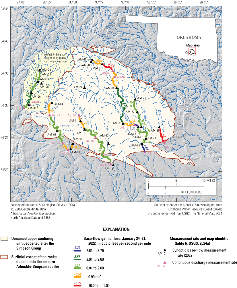
Synoptic base-flow measurement sites and gaining and losing stream reaches crossing the surficial extent of the rocks that contain the eastern part of Arbuckle-Simpson aquifer, south-central Oklahoma, January 24–31, 2022.
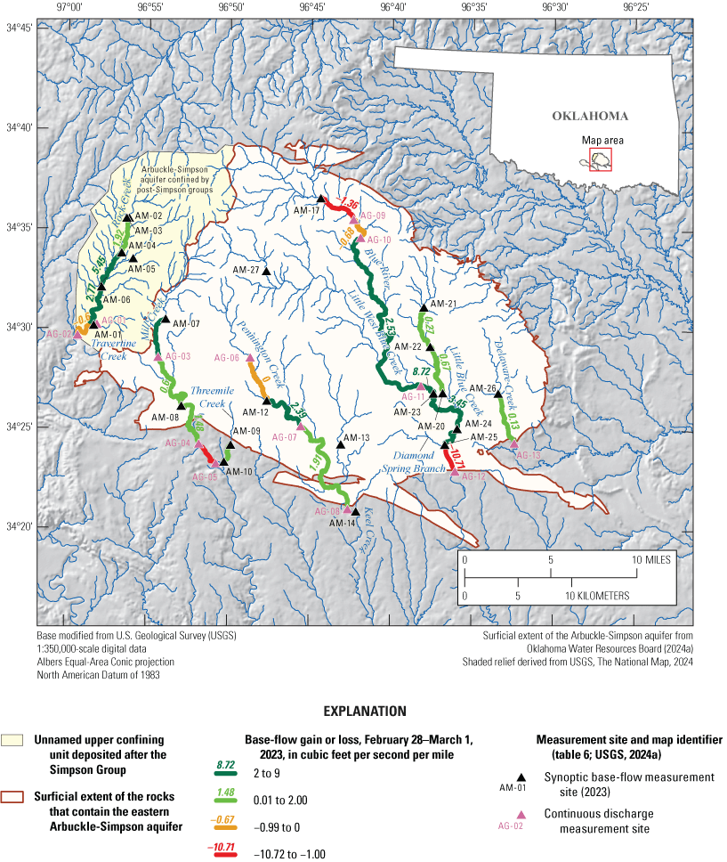
Synoptic base-flow measurement sites and gaining and losing stream reaches crossing the surficial extent of the rocks that contain the eastern part of Arbuckle-Simpson aquifer, south-central Oklahoma, February 28–March 1, 2023.
Discrete discharge measurements, referred to as synoptic base-flow measurements (seepage runs), were made at several sites along streams during a period of relatively low precipitation in a short period of time to determine base flow. Synoptic base-flow measurements were collected by using the methods of Rantz and others (1982) and Turnipseed and Sauer (2010). Each streamflow measurement was assigned a quality rating by the field technician. The following ratings were assigned to measurements based on USGS guidelines (Turnipseed and Sauer, 2010): excellent, measured discharge was within 2 percent of actual discharge; good, measured discharge was within 5 percent of the actual discharge; fair, measured discharge was within 10 percent of the actual discharge; poor and unspecified, measured discharge was assumed to be within 8 percent of actual discharge (table 6). Gaining and losing segments were determined by calculating the difference in seepage (streamflow discharge) measurements at each end of a segment. To calculate a rate of gain or loss per mile along the segment, the difference in discharge was divided by the stream length between the upstream and downstream measurement. Base flow increases in the downstream direction in a gaining stream as water seeps into the stream from the aquifer, whereas base flow decreases in the downstream direction in a losing stream as water seeps out of the stream to the aquifer (Winter and others, 1998). Tributary inflow was accounted for in these measurements by subtracting tributary discharge from the upstream measurement.
The 2022 seepage measurements indicated net gaining stream reaches along portions of Rock Creek, Mill Creek, Pennington Creek, and the Blue River (fig. 8). Net gaining stream reaches indicate that groundwater from the Arbuckle-Simpson aquifer is flowing into streambeds and maintaining streamflows. Upstream reaches of the Blue River to the north of site AM-18 were net losing; streamflows ranged from 0.00 to 4.28 ft3/s in these reaches, indicating net seepage losses from the stream into the Arbuckle-Simpson aquifer. Streamflows measured between sites AM-18 and AM-19 indicated a gain of 2.33 ft3/s per mile. Streamflow measured at the Blue River streamgage (site AG-12) and the measurement upstream at site AM-25 indicated a gain of 7.63 ft3/s per mile. There was no flow in the upper reach of Pennington Creek upstream from site AG-06 or between the next two downstream seepage measurement sites AM-11 and AM-12. There was no flow in Mill Creek upstream from sites AM-07 and AG-03, but there was streamflow between sites AG-03 and AG-04, and in this reach streamflow increased by 0.27–0.28 ft3/s per mile. Delaware Creek lost streamflow between sites AM-26 and AG-13. Little Blue Creek, a tributary to the Blue River, gained streamflow of 0.26 ft3/s per mile between sites AM-21 and AM-20.
The 2023 seepage measurements indicated that more stream segments were gaining than during the 2022 seepage measurements on Mill Creek, Pennington Creek, Blue River, Little Blue Creek, and Delaware Creek (fig. 9). In addition, streamflows computed at USGS streamgages in the study area were generally greater during February 28–March 1, 2023, than during January 24–31, 2022. For example, streamflow values at sites AG-09 and AG-10 during 2022 were both 0.0 ft3/s, but streamflow values during 2023 at those streamgages were 12.7 and 11.5 ft3/s, respectively.
Springflow Monitoring
Springs are a common feature of karst aquifers, and numerous springs issue from the eastern part of the Arbuckle-Simpson aquifer (OWRB, 2003). Spring discharge measurements were collected by using the same methods as described for the streamflows in the “Streamflow Monitoring” section of this report. Springs are points or areas of natural outflow of groundwater to the land surface. Where this groundwater discharges from the Arbuckle-Simpson aquifer, groundwater can discharge downstream to join a stream, can re-enter the aquifer if karstification continues downgradient, or can be naturally dammed to create a pond, such as the pond that was formed in the 1870s by damming Byrds Mill Spring, which was later enclosed in 1927 in a cement and metal structure (OWRB, 2007). In addition, when groundwater discharges to the land surface, especially if it flows into a pond that is not enclosed, some of that water will be lost to evaporation.
Continuous Springflow Monitoring
Discharge was continuously monitored at USGS streamgages at four major springs in the study area: Antelope Spring, unnamed Blue River spring, Byrds Mill Spring, and Sheep Creek Spring (fig. 2). Byrds Mill Spring near Fittstown, Okla. (07334200; table 1–1 in appendix 1) was monitored during 1959–2017 at the Byrds Mill Spring gage; data were used in the Phase 1 analyses, but this gage was discontinued prior to the initiation of the Phase 2.
Seasonal patterns were observed in spring discharge. Spring discharge was generally lower in summer and winter when there is typically less precipitation compared to fall and spring, and evaporation losses reach their annual peak in the summer, which also causes spring discharge to decrease relatively more than during other seasons. For all seasons, spring discharges were generally highest during the spring because seasonal precipitation amounts are highest and because evapotranspiration rates in the spring are relatively low compared to those in the summer.
Continuous spring discharge hydrographs from the Antelope Spring gage, Byrds Mill Spring gage (USGS streamgage 07334200), and Sheep Creek Spring gage were analyzed for the highest discharge periods during 2015–16 to identify flow regimes of this karst aquifer. Linear regression equations (regression curves) for spring discharge and time were examined for breaks (inflection points) in the recession slope, which are indicative of a change from one flow regime to another within the karst continuum (Otero, 2007). Diffuse flow is the amount of water that flows through the rock matrix (Kresic, 2013). Conduit flow is the amount of water that flows through rock fractures or conduits, which are interconnected solution cavities where the length is disproportionally larger than the height or width (Kresic, 2013). Recession curves were classified as different flow regimes based on their decay coefficient (α) in Milanović’s (1976) equation:
whereQt
is discharge at time t, in cubic feet per second;
Q0
is initial discharge, in cubic feet per second;
e
is a mathematical constant equal to approximately 2.71828; it is the base of the natural logarithm and of its related inverse, the exponential function;
t
is time, in seconds; and
t0
is time at the beginning of each recession slope, in seconds.
If the decay coefficient is 0.18, then conduit flow is the predominant flow type. If the decay coefficient is 0.09, then flow type consists of fracture flow or a mixture of conduit flow and diffuse flow (with conduit dominant). If the decay coefficient is 0.02, then flow type consists of fracture flow or a mixture of conduit flow and diffuse flow (with diffuse dominant). If the decay coefficient is 0.008, the diffuse flow is the predominant flow type (Milanović, 1976). As indicated by the recession curves at the highest discharge periods, Antelope Spring yielded a higher decay coefficient than during the other periods of recession and exhibited more conduit flow than diffuse flow, followed by greater portions of mixed and diffuse flow (fig. 10A). This higher decay coefficient indicates that during periods of high-discharge recession, the groundwater system supplying Antelope Spring might include upper layers of the aquifer dominated by fractures and conduits, with a middle and lower section of the aquifer dominated by fractures, primary porosity, or both.
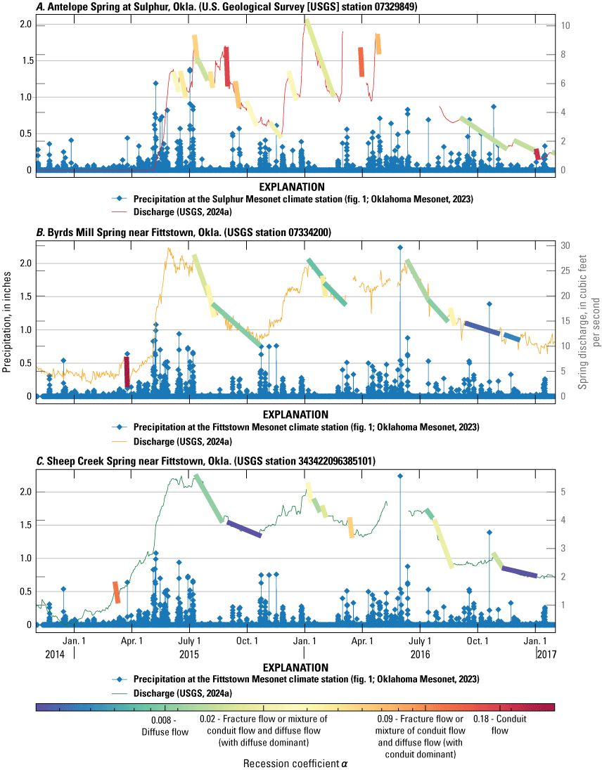
Discharge and spring recession curves classified by flow regime and precipitation for A, Antelope Spring, B, Byrds Mill Spring, and C, Sheep Creek Spring, south-central Oklahoma, 2014–17.
As indicated by recession curves for the highest discharge periods for the Byrds Mill Spring and Sheep Creek Spring gages, decay coefficients are relatively lower and flow is mostly diffuse compared to Antelope Spring (fig. 10B, C). These lower decay coefficients indicate that the groundwater system near Byrds Mill and Sheep Creek Springs, near the upper levels of the formation, is likely dominated by diffuse drainage through primary porosity.
Discrete Springflow Measurements
Discrete springflow measurements were made during 2022–23 at springs in the study area (table 1–2 in appendix 1) to document current springflows (at the time when the measurements were made) across the eastern part of the Arbuckle-Simpson aquifer for the Phase 2 study and to better understand changes in springflow over time (table 7). As explained in the “Introduction” section of this report, changes in the springflow over time across the aquifer could be an indicator of change in aquifer water storage amounts. Spring discharges were not measured and documented specifically for the Phase 1 studies, but historical spring discharges from the USGS NWIS database (1954–2017) (USGS, 2024a) were analyzed by the OWRB to identify which springs to include for the well-spacing rules for sensitive sole-source groundwater basins. Spring discharges for Phase 2 were measured during 2018–23, with some multiple measurements for the Phase 2 period of record specified in table 8 to indicate the period for which the Phase 2 mean discharge was calculated. The OWRB well-spacing rules are dependent on springs flowing greater than 50 gal/min (0.11 ft3/s) and 500 gal/min (1.11 ft3/s). Springflows as determined from historical discharge measurements were compared to Phase 2 discharge measurements (table 7). Eleven of the 17 spring sites had a decrease in discharge from the historical period to Phase 2 (table 7). Additional spring locations were documented, and discharge was measured for Phase 2 (table 1–2, appendix 1).
Table 7.
Differences in mean discharge at spring sites between historical period of record and 2018–23 (Phase 2), eastern part of the Arbuckle-Simpson aquifer, south-central Oklahoma.[USGS, U.S. Geological Survey; ft3/s; cubic feet per second. Data are from USGS (2024a)]
Groundwater Monitoring
Groundwater-level data were collected in accordance with methods described in Cunningham and Schalk (2011). The Cunningham and Schalk report documents field methods for the establishment of a permanent measuring point and of other reference marks for a well site, how to measure water levels using steel tapes and electric tapes, how to monitor continuous water levels with a pressure transducer, and how to test if a well is in connection with the aquifer. These methods described by Cunningham and Schalk are standard operating procedures used by the USGS for accuracy and verification of groundwater-level data collected.
The continuous groundwater monitoring network that was established for Phase 2 consisted of 23 wells, with 18 wells completed in the Arbuckle Group and 5 wells completed in the Simpson Group (table 8). Six of the wells for Phase 2 were also used in Phase 1 for continuous groundwater levels monitoring. Groundwater-level data from Phase 1 were compared to those collected during Phase 2 at five wells, with the results indicating relatively unchanged mean groundwater levels (fig. 11). The periods of lowest groundwater levels (the “troughs” on the groundwater-level hydrographs) typically occurred during the summer and winter months, and the troughs were generally shallower during Phase 2 than during Phase 1. The peaks on the groundwater-level hydrographs (typically during the spring and fall months) during Phase 1 were sometimes slightly shallower or deeper or relatively unchanged compared to those of Phase 2. The mean depth of the wells being monitored in conjunction with this study that are completed in the portion of the eastern part of the Arbuckle-Simpson aquifer contained in the Arbuckle Group is 190 ft bls, excluding one well where the depth is approximately 920 ft bls (table 8). The mean depth of the wells being monitored in conjunction with this study that are completed in the portion of the eastern part of the Arbuckle-Simpson aquifer contained in the Simpson Group is 120 ft bls.
Table 8.
Periods of record for continuous groundwater monitoring wells completed in the Arbuckle or Simpson Group across the eastern part of the Arbuckle-Simpson aquifer, south-central Oklahoma.[USGS, U.S. Geological Survey; bls, below land surface. Phase 1 refers to data collected primarily during 2003–02, and Phase 2 refers to data collected primarily during 2018–23. Data are from USGS (2024a). Dates are in year-month-day format. --, no data]
OWRB ID 89386 during Phase 1 study (Christenson and others, 2011).
OWRB ID 89387 during Phase 1 study (Christenson and others, 2011).
OWRB ID 92477 during Phase 1 study (Christenson and others, 2011).
OWRB ID 93617 during Phase 1 study (Christenson and others, 2011).
OWRB ID 86266 during Phase 1 study (Christenson and others, 2011).
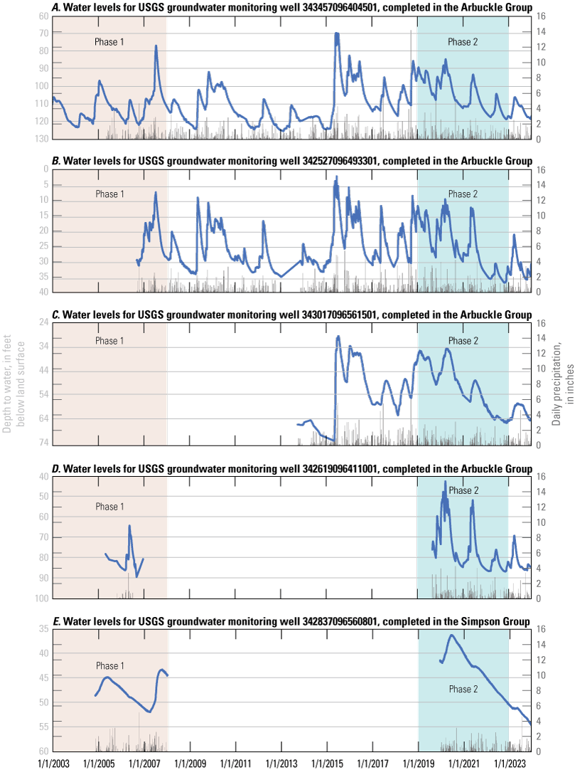
Depth to water and daily precipitation for U.S. Geological Survey (USGS) monitoring wells completed in the A–D, Arbuckle Group and E, the Simpson Group, south-central Oklahoma, 2003–23.
The Arbuckle Group is exposed at the surface through most of the study area, and the part of the Arbuckle-Simpson aquifer contained in these rocks is primarily recharged through precipitation. The karstic nature of the aquifer allows for a somewhat flashy response in groundwater levels because recharge can flow quickly through conduits through fractures and along faults (Fairchild and others, 1990). Wells completed in the Arbuckle Group typically yield 200 to 500 gal/min (Fairchild and others, 1990). Water levels measured in wells completed in the Arbuckle Group are more variable compared to the water levels measured in wells completed in the Simpson Group; the variability in water levels is caused by seasonal changes in water use, precipitation, and evaporation, along with other seasonal changes.
The Simpson Group is exposed at the surface in the western part of the study area, as well as a small section in the southeastern part of the study area (fig. 2). The Simpson Group is less karstic than the Arbuckle Group and primarily stores and transports water through diffuse flow via pore spaces in the sandstones that are part of the Simpson Group (Fairchild and others, 1990; Christenson and others, 2011). Flow through pore spaces is slower than flow through conduits and karst features, and as a result, groundwater levels in the Simpson Group respond to precipitation in a more subdued, less flashy way. The less karstic nature of the Simpson Group also lends itself to lower well yields than the Arbuckle Group, typically 100 to 200 gal/min (Fairchild and others, 1990; Christenson and others, 2011).
Wells completed in the part of the aquifer contained in either the Arbuckle or Simpson Group exhibit seasonal changes and patterns in water levels. During the spring and fall, when precipitation is seasonally at its highest, the water levels in both aquifers tend to be higher compared to water levels during the winter and summer months. During the summer, water levels tend to be lower than in any of the other seasons because of less precipitation and increased water use and evapotranspiration; summer is when most groundwater is withdrawn for crop irrigation, lawn watering, and other activities such as filling swimming pools, washing cars, and watering gardens. Water levels in the study area during the summer and winter, particularly in the Arbuckle Group of the Arbuckle-Simpson aquifer, appeared to be generally decreasing during Phase 2. These declining water levels were most likely caused by decreasing precipitation (fig. 11) but could also have been caused by increased water use or evapotranspiration.
Potentiometric Surfaces
A potentiometric surface is a surface of equal hydraulic head or potential, typically depicted by a map of equipotential lines such as water-table elevations (Sharp, 2024) and thus represents a snapshot of groundwater levels (commonly referred to as the water table) across the aquifer for a specific point in time. Specific points on potentiometric-surface maps are roughly equivalent to the level to which water will naturally rise in a tightly cased well. Potentiometric-surface maps can be used to help identify groundwater-flow directions, delineate subsurface groundwater basins, and estimate changes in groundwater storage by comparing potentiometric surfaces from different time periods (Driscoll, 1986). The altitudes of potentiometric surfaces of the Arbuckle-Simpson aquifer were calculated by collecting groundwater-level measurements at 57 groundwater wells across the study area in 2022 (fig. 12) and 56 wells in 2023 (fig. 13). These measurements were collected during base-flow conditions in mid-February 2022 and 2023, when evapotranspiration rates and groundwater use are less compared to other months.
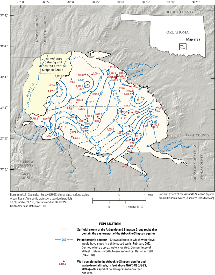
Potentiometric surface of the eastern part of the Arbuckle-Simpson aquifer, south-central Oklahoma, February 2022.
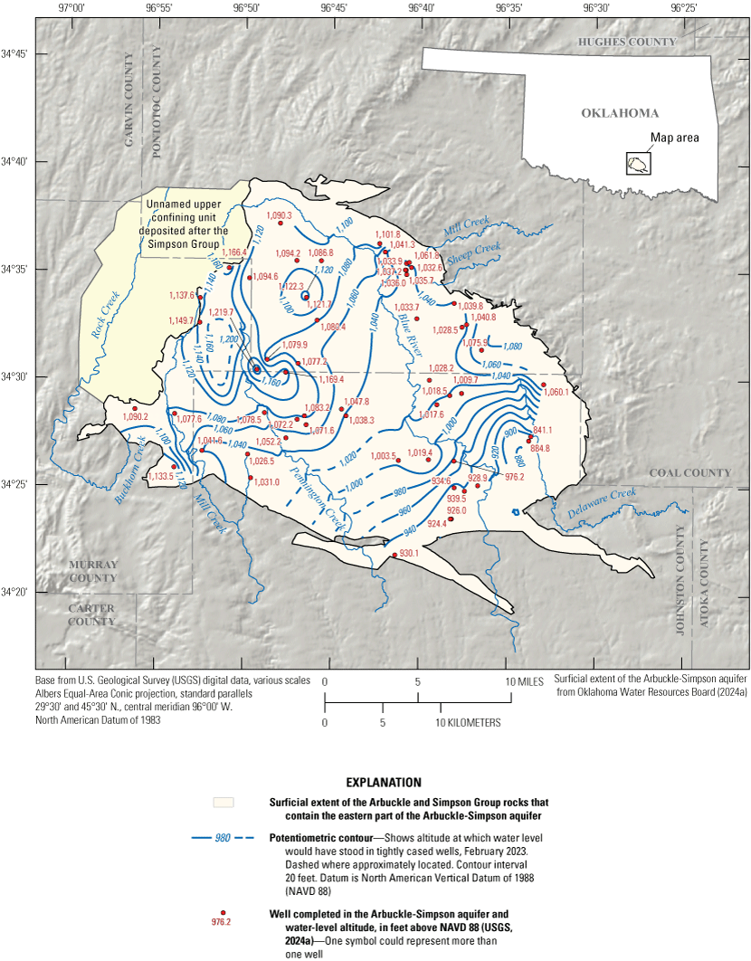
Potentiometric surface of the eastern part of the Arbuckle-Simpson aquifer, south-central Oklahoma, February 2023.
A potentiometric surface is a theoretical topographical surface which represents the fluid potential of groundwater within an aquifer. Potentiometric surfaces were constructed in ArcGIS Pro by combining synoptic water-level data with a digital elevation model (DEM) and generating contours around the derived static head measurements (depth to water, in feet below land surface datum). Contours were adjusted to remedy irregularities resulting from automated contour generation and known inconsistencies in the study area. The resultant map displays a surface that can be used to interpret the direction groundwater will flow throughout a given aquifer.
Groundwater-level data were used to create two potentiometric-surface maps over the main area of the eastern part of the Arbuckle-Simpson aquifer (figs. 12–13). Both maps show a decrease in water-level altitude from the northwest to the southeast indicating the general direction of groundwater flow through the aquifer while also displaying some variation from year to year. Despite some fluctuations, potentiometric surfaces for the Arbuckle-Simpson aquifer indicate that regional groundwater flow is toward the southeast, where streams and springs discharge at the aquifer boundary, which is consistent with the findings of Christenson and others (2011).
Water-level altitude measurements used for the 2022 potentiometric surface ranged from 861 to 1,163 ft above the North American Vertical Datum 1988 (NAVD 88), with a mean of 1,039 ft above NAVD 88 (USGS, 2024a). Water-level altitudes used for the 2023 potentiometric surface ranged from 885 to 1,220 ft above NAVD 88, with a mean of 1,050 ft above NAVD 88. Although the variance and difference in mean values from 2022 to 2023 are not substantial, the mapped potentiometric contours have differences. The largest differences in water-level altitudes between 2022 compared 2023 are in an area containing four wells east of Pennington Creek. The water-level altitudes were higher in 2023 than in 2022: 1,086.8, 1,081.9, 1,092.3, and 1,092.5 ft above NAVD 88 for 2022 and 1,079.9, 1,077.2, 1,169.4, and 1,219.7 ft above NAVD 88 for 2023, respectively. Even with other examples of localized differences between the two maps, general patterns remained similar in 2022 and 2023.
In Phase 1, three potentiometric-surface maps were prepared and analyzed. The measurements used to generate these maps were collected during August 7–16, 1995; June 2006; and September 2006 (Christenson and others, 2011). As expected, these maps feature a slope from a topographic high between Blue River and Pennington Creek just east of the confined part of the eastern Arbuckle-Simpson aquifer to the southeast. This slope to the southeast from a topographic high is common to all Arbuckle-Simpson potentiometric-surface maps. Although this overarching pattern holds true as illustrated for Phase 1 and Phase 2 maps (figs. 12–13), localized variations for different time periods were observed.
The three potentiometric-surface maps produced for Phase 1 exhibit contours that “V” upstream near Delaware Creek in the southeast part of the main aquifer area (figs. 18–20 in Christenson and others, 2011). This “V” of contours is still slightly indicated but is harder to detect in the Phase 2 potentiometric-surface maps (figs. 12, 13) compared to those from Phase 1. This difference in prominence of contours could be due to the higher density of measurements in this area in Phase 1 that allowed detection of smaller scale features. This interpretation of the effects of measurement density on the ability to detect smaller scale features can be extended to other differences between the potentiometric surface; approximately 90 groundwater-level measurements were used to create the 2006 map compared to 57 and 56 groundwater-level measurements used for the 2022 and 2023 maps, respectively.
Across the eastern part of the Arbuckle-Simpson aquifer, groundwater levels were slightly higher in altitude (nearer the ground surface) during Phase 2 compared to Phase 1. The variation in the potentiometric surfaces between Phase 1 and Phase 2 could be attributed to the time at which measurements were collected. For Phase 2, water levels were measured February 14–17, 2022, and February 13–16, 2023, during base-flow conditions. Collecting groundwater-level measurements during base-flow conditions reduces effects from evapotranspiration, peak water use, and precipitation. In contrast to the Phase 2 groundwater levels, Phase 1 groundwater levels were not measured during base-flow conditions.
Recharge
Even though aquifer recharge can be a result of many different processes or a combination of processes, the dominant recharge mechanism for the eastern part of the Arbuckle-Simpson aquifer is infiltration of precipitation through the soil. This precipitation recharge takes place when precipitation falls on the land surface and subsequently percolates into the unsaturated zone. Evapotranspiration is the combination of evaporation and transpiration, with evaporation being water that transpires from a surface to the atmosphere and transpiration being water taken up by plants and released as vapor into the atmosphere (Sharp, 2024). The amount of precipitation that successfully infiltrates into soil and passes through an unsaturated zone for recharge to the water table is dependent on many factors such as the amount of water stored in the unsaturated zone, the slope of the land surface, the composition of the rocks and soils that form the aquifer, the type of vegetation and general land use overlying the aquifer, and the intensity, season, and duration of precipitation. Owing to the substantial number of variables that affect recharge via infiltration from precipitation, estimates are difficult to quantify. Two methods were used in this study to estimate recharge: (1) a recession-curve displacement method, referred to as the RORA method (Rorabaugh, 1964; Rutledge, 1998) and implemented as the RORA program, was used to estimate recharge in a watershed upstream from a selected streamgage, and (2) the Soil-Water-Balance (SWB) code (Westenbroek and others, 2010) was used to model spatially distributed recharge rates across the aquifer.
RORA Recession-Curve Displacement Method
For Phase 1 and Phase 2, the basin-scale recession-curve displacement method developed by Rorabaugh (1964) that was implemented in the USGS Groundwater Toolbox as the “RORA program” (Barlow and others, 2015) was used to estimate recharge within watersheds upstream from selected streamgages in the eastern part of the Arbuckle-Simpson aquifer (Rorabaugh, 1964; Rutledge, 1998). The RORA program is used to estimate the change in the total potential groundwater discharge (base flow) at a critical time after the peak (peak in streamflow caused by higher rates of precipitation and runoff) by extrapolation from the pre-peak and the post-peak recession periods (Rutledge, 1998). Recharge from each precipitation event is assumed to be the difference between the groundwater discharge to the stream and the groundwater discharge that would have happened at the same time in the absence of the recharge event, based on extrapolation of the streamflow hydrograph prior to the recharge event. Recharge commonly is divided by the area of the drainage basin and expressed as a rate in inches per year. The areas of the subsurface watersheds (Christenson and others, 2011, fig. 21 and table 8) were used as the watershed areas for this study. Owing to assumptions and stipulations inherent to this method of recharge estimation, three USGS streamgages were selected by Christenson and others (2011) for analysis in a Phase 1: the Blue River streamgage (table 9), the Pennington Creek near Reagan gage (table 10), and Honey Creek below Turner Falls near Davis (USGS streamgage 07329780). The Honey Creek below Turner Falls near Davis streamgage is not located in the eastern part of the Arbuckle-Simpson aquifer and therefore is not listed in table 9 or 10. The period of record analyzed for recharge for the Blue River streamgage (table 9) for phase 1 included the years 1977–79 and 2004–08. The period of record analyzed for recharge for the Pennington Creek near Reagan streamgage (table 10) for phase 1 included the years 2004–2008. These sites were used in Phase 2 to allow for direct comparison and discussion of temporal variations. The USGS Groundwater Toolbox programs RECESS (Rutledge, 1998) and RORA (Barlow and others, 2015) were used in conjunction with streamgage data to compute the recharge values shown in tables 9 and 10. The use of these tools is elaborated upon in Christenson and others (2011).
Table 9.
Quarterly recharge calculated for U.S. Geological Survey streamgage 07332390 at Blue River near Connerville, Oklahoma, for Phase 1 (1977–2008) and Phase 2 (2018–22) periods.[Subsurface watershed area (from fig. 21 and table 8 in Christenson and others, 2011) using the basin-scale recession-curve displacement method (Rorabaugh, 1964; Rutledge, 1998); Phase 1 mean values include only the water years during 1977–2008 that are listed in this table; Phase 2 mean values are for water years 2018–22]
Table 10.
Quarterly recharge calculated for U.S. Geological Survey streamgage 07331300 at Pennington Creek near Reagan, Oklahoma, for Phase 1 (2004–08) and Phase 2 (2018–22).[Subsurface watershed area (from fig. 21 and table 8 in Christenson and others, 2011) using the basin-scale recession-curve displacement method (Rorabaugh, 1964; Rutledge, 1998); Phase 1 mean values include only the water years during 2004–08 that are listed in this table; Phase 2 mean values are for water years 2018–22]
The mean annual estimated recharge determined by using the RORA program for the eastern part of the Arbuckle-Simpson aquifer was 16.5 inches per year (in/yr; 43 percent of the 37.97 inches of mean annual precipitation) during 2018–22. Phase 2 mean annual recharge determined by using the RORA program was greater than Phase 1 mean annual recharge at the same two sites measured and analyzed for Phase 1 and Phase 2. For the Blue River streamgage, the mean annual recharge increased by 98 percent from Phase 1 to Phase 2. For the Pennington Creek near Reagan gage, the mean annual recharge increased by 33 percent from Phase 1 to Phase 2.
Upstream anthropogenic streamflow augmentation from producing mines affects recharge estimates obtained from the RORA program by increasing the part of the hydrograph that is interpreted by the RORA program as recharge to the aquifer (fig. 7). Because these augmentations to streamflow were not measured and are difficult to estimate and separate from the streamflow hydrograph, the estimates of recharge derived by the RORA program are likely overestimated for basins where these releases occurred.
Soil-Water-Balance Code
The SWB (Westenbroek and others, 2010) code was run to estimate the amount and spatial distribution of daily groundwater recharge to the eastern part of the Arbuckle-Simpson aquifer only for the years from 2019 through 2022 of the Phase 2 period because most of the groundwater well data collection in Phase 2 started in 2019 (table 8). At the time the SWB code was run for this report, the climate data for 2023 were not available yet. SWB is a modified Thornthwaite and Mather (1957) SWB method that uses gridded climate data and landscape characteristics to calculate recharge by using the following equation:
whereR
is recharge, in inches per day;
P
is precipitation, in inches per day;
S
is snowmelt, in inches per day;
Ri
is surface runoff inflow, in inches per day;
Int
is plant interception, in inches per day;
Ro
is surface runoff outflow, in inches per day;
Pet
is potential evapotranspiration, in inches per day; and
ΔSm
is the change in soil moisture, in inches per day.
Data inputs that are used in the SWB code include precipitation, air temperature, soil-water storage capacity, hydrologic soil group, land-surface flow direction, and land-cover type. The user-specified grid for the eastern part of the Arbuckle-Simpson aquifer SWB code consisted of 2,180 columns by 1,831 rows of cells that were each 328 by 328 ft. Climate data inputs included daily grids of precipitation data and minimum and maximum air temperature during 2019–22 from the Daymet climate database (Thornton and others, 2024). Soil properties (soil-water storage capacity and hydrologic soil group) were obtained from the gridded Soil Survey Geographic database (U.S. Department of Agriculture, 2024). Land-cover types were obtained from the National Land Cover Database (Multi-Resolution Land Characteristics Consortium, 2024) and resampled to the SWB model grid resolution by using the most common land-cover type within each cell. Surface runoff was derived by using the D8 method (Greenlee, 1987) to calculate the land-surface gradient from a 10-meter DEM (USGS, 2015). Depressions were filled by using the ArcGIS Fill tool (Esri, 2024) after the DEM was resampled to the SWB model grid size. Filling depressions in the DEM ensures correct routing of surface runoff and eliminates isolated sink features that would result in unrealistically high amounts of recharge.
The Hargreaves and Samani (1985) method for calculating evapotranspiration was used for a reference latitude of 34.240000 to 34.740000 degrees. Land-cover types were used in conjunction with hydrologic soil groups to partition daily precipitation into plant interception (Int) and surface runoff (Ri and Ro) components and assign plant root-zone depths. The root-zone depths for grassland/herbaceous and pasture (the dominant land-cover types in the study area) varied with soil texture but ranged from about 0.8 to 1.5 ft. The maximum volume of water available in the root zone was calculated by multiplying the soil-water storage capacity by the root-zone depth. Changes in soil moisture (ΔSm) exceeding the soil-water storage capacity were assumed to be recharge (R) to the saturated zone. Smaller root-zone depths resulted in increased recharge and decreased evapotranspiration of water from the root zone whereas larger root-zone depths resulted in decreased recharge and increased evapotranspiration of water from the root zone. Recharge from irrigation was not simulated by SWB but was assumed to be negligible given the relatively small amount of irrigation groundwater use in the study area.
Recharge from precipitation was assumed to occur where the eastern part of the Arbuckle-Simpson aquifer is unconfined. The portion confined by the post-Simpson Pennsylvanian units was analyzed by using the SWB code but was not included in the mean recharge calculation for the study area (fig. 14). The mean annual SWB-estimated recharge for the eastern part of the Arbuckle-Simpson aquifer was 4.85 in/yr (or 13 percent of the 37.97 inches of mean annual precipitation) for the 2019–22 period (fig. 4A). The annual SWB-estimated recharge for the eastern part of the Arbuckle-Simpson aquifer was 7.2 inches for 2019, 5.9 inches for 2020, 2.6 inches for 2021, and 3.6 inches for 2022. Mean annual recharge estimated by using the RORA program for Phase 2 (2018–22) was 16.5 in/yr, which is greater than the mean annual recharge of 4.85 in/yr estimated by using SWB for Phase 2 (2019–22).
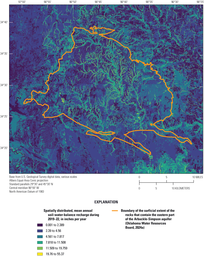
Spatially distributed mean annual recharge computed by using the Soil-Water-Balance code (Westenbroek and others, 2010) for the eastern Arbuckle-Simpson aquifer study area, south-central Oklahoma, 2019–22.
The SWB code cannot be used to simulate interactions between surface-water and groundwater features. In locations where the water table is beneath the bottom of the root zone, the SWB code can be used to produce reasonable annual or monthly values. The depth from the bottom of the root zone to the top of the water table is not considered in the estimation of recharge because there may be appreciable travel time through the unsaturated zone. Simulating the unsaturated zone was outside the scope of this project. Using the SWB code in areas with wetlands, springs, and lakes where the water table is close to the land surface produced unrealistic annual or monthly values because there is no provision for recharge rejection in the form of saturation excess (other than a maximum recharge rate that can be specified for a land use and soil type). Because the eastern part of the Arbuckle-Simpson aquifer is a karst aquifer, recharge estimates obtained by using the SWB code were compared with estimates obtained by using other recharge methods (such as the RORA program). SWB code can nonetheless be used to create reliable spatially gridded recharge estimates for the study area with spatial variations in recharge across different surficial features of the eastern part of the Arbuckle-Simpson aquifer. The alluvial sediments and soils near streams have higher recharge rates than the surrounding soil types overlying the Arbuckle and Simpson Groups that make up the eastern part of the Arbuckle-Simpson aquifer (fig. 14).
Groundwater Withdrawals and Water Use
Permitted users of groundwater in Oklahoma are required by statute to report their water use annually to the OWRB (Oklahoma State Legislature, 2023d). The OWRB does not require permits for the following: use of water by a natural individual or by a family or household for household purposes, for farm and domestic animals up to the normal grazing capacity of the land whether or not the animals are actually owned by such natural individual or family, and for the irrigation of land not exceeding a total of three acres in area for the growing of gardens, orchards, and lawns. Domestic use also includes: (1) the use of water for agriculture purposes by natural individuals, (2) use of water for fire protection, and (3) the use of water by non-household entities for drinking water purposes, restroom use, and the watering of lawns, provided that the amount of groundwater used for any such purposes does not exceed five acre-feet per year. Pit dewatering is exempt from needing a permit unless the mine (pit) is overlying the Arbuckle-Simpson aquifer.
Most groundwater wells currently (2024) completed in the eastern part of the Arbuckle-Simpson aquifer are primarily for domestic use, with agriculture as the second most common type of use. The depths of most wells completed in the eastern part of the Arbuckle-Simpson aquifer are less than 200 ft bls, and in general, wells completed in the part of the eastern part of the Arbuckle-Simpson aquifer contained in the Simpson Group tend to be shallower than those completed in the Arbuckle aquifer, where well depths can be as much as 800 ft bls.
Groundwater Withdrawals
The amount of groundwater that can be appropriated in Oklahoma is tied to the amount of land the applicant either owns or leases and the equal proportionate share determined by the OWRB for the underlying aquifer (Oklahoma State Legislature, 2023b). These lands put toward the application are referred to as “dedicated lands” (fig. 1). Groundwater-use data are self-reported by the permitted groundwater user annually to the OWRB. Nine different beneficial groundwater-use types are regulated by the OWRB for groundwater permits: (1) irrigation, (2) public supply, (3) industrial, (4) power, (5) mining, (6) commercial, (7) recreation, fish, and wildlife, (8) agricultural, and (9) other (fig. 1). Power and commercial groundwater-use type was not included in this study’s results because of no reported use in that category. The amounts of groundwater used for recreation, fish, and wildlife, agriculture, and other have been combined into one category because of their relatively low combined use amount compared to the other uses. Public supply was the most reported beneficial groundwater-use type during 1967–2020 for the eastern part of the Arbuckle-Simpson aquifer, with the aquifer providing water for municipalities within the study area (fig. 15A; table 11; Mashburn and others, 2025). The mean annual reported groundwater use during 1967–2020 was 3,251 acre-feet.
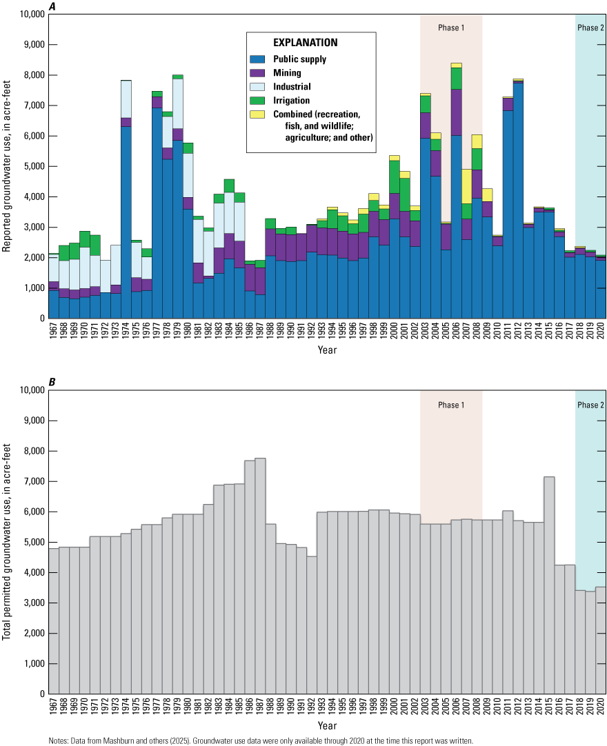
A, Reported groundwater use by type and B, permitted groundwater use during 1967–2020 for the eastern part of the Arbuckle-Simpson aquifer, south-central Oklahoma.
Table 11.
Annual reported groundwater use during 1967–2020 for the eastern part of the Arbuckle-Simpson aquifer, south-central Oklahoma.[Values are shown in the reported precision and are in units of acre-feet; Power and commercial groundwater-use types not listed because of zero reported groundwater use; Data are from Mashburn and others (2025)]
Permitted amounts per groundwater user were summed for each year (fig. 15B). Some permitted groundwater users did not report use each year, which could be because of not using their permitted allotment or they were not compliant with reporting requirements. For example, the City of Ada reported groundwater use of 4,179 and 5,094 acre-feet in 2011 and 2012, respectively, with little (less than 1,100 acre-feet) to no groundwater use reported during 2013–20. As described in Christenson and others (2011, p. 51),
The large variation in reported groundwater use by the City of Ada is largely related to variation in discharge from Byrds Mill Spring, Ada’s primary water source. When discharge from Byrds Mill Spring is adequate to meet demand, the City of Ada meets that demand by diverting water from the spring and does not withdraw groundwater. Water diverted from Byrds Mill Spring is reported as surface-water use, and therefore, in years when the flow from Byrds Mill Spring is adequate to meet demand, Ada’s reported groundwater use is zero. When discharge from the spring is low, Ada supplements water from the spring by withdrawing groundwater from wells completed in the aquifer to preserve streamflow for downstream landowners.
Consumptive Water Use at Producing Mines
Additional rules related to the withdrawal, use, and disposal of groundwater associated with producing mines provide a framework to protect groundwater in the Arbuckle-Simpson aquifer (Oklahoma State Legislature, 2023e). Based on these rules, the OWRB gathers data provided by the mining companies of monitoring and periodic reporting of groundwater disposition. Mines are required by the OWRB to submit either a management plan to monitor and quarterly and annual reports of water volumes. These management plans and reports include a water budget for the mine that describes anticipated water moving into and out of the mine site as stream and groundwater inflows and outflows (includes augmentation outflows to streams and the groundwater system), pit water, precipitation runoff, and evaporation. These water volumes are used by the OWRB to estimate the consumptive use of pit water.
Water volume data from these management plans and reports were compiled for 2019–22 from the OWRB website (OWRB, 2024b) in February 2024. Each mine is required to report these data once every quarter, as well as a total annual water volume. Each mine is required to report the amount of precipitation that falls onto the land and flows over the land surface and subsequently drains into mine pits, as well as nonconsumptive water losses (including pit water returned to the land surface from which surface runoff flows into a mine pit). Some of the mines, are considered de minimis, that coincide with the location of the eastern part of the Arbuckle-Simpson aquifer have an exemption from having to report the measured quarterly or annual water volumes, but they are still required to submit a plan of anticipated volumes. De minimis is the taking, use or disposal of pit water in an amount less than five acre-feet per year (Oklahoma State Legislature, 2023b). For the purposes of this study, water volumes provided per mine in either a management plan or a quarterly or annual report were included in the estimated consumptive use. The consumptive use estimates do not distinguish between groundwater and surface water. Some reports appeared to be incomplete; however, it was beyond the scope of this report to resolve any apparent discrepancies in reported water volumes.
Consumptive use water volumes were compiled from annual plans and reports for the 2019–22 period for eight mines (table 12). Of the 11 mines that submitted reports to the OWRB, 3 of them indicated that they had no water volume to report (OWRB, 2024b). Three of the remaining eight mines that submitted reports coincide with the surficial extent of the eastern part of the Arbuckle-Simpson aquifer (table 12). A negative consumptive water-use value indicates that there was no consumption of water by the mine and water was returned to the natural system through a variety of processes that exceeded the total volume of water withdrawn from the producing mine pit (mine pit pumping), including natural evaporation from the pit, water evaporated during the drying of the mined material, water in the mined material transported from the mine, volume of water used for beneficial uses, pit water returned to a groundwater basin (groundwater augmentation), pit water returned to a definite stream during flow conditions that are less than or equal to 50-percent exceedance (stream augmentation) (fig. 7), and other losses such as pit groundwater returned to the land surface via runoff. The 50-percent exceedance is the median of mean daily flows for the period of record analyzed (Oklahoma State Legislature, 2023b). The USGS streamflow data are used by the OWRB to update the calculation of the 50-percent exceedance annually. Mines can offset the water pumped from the mine if stream augmentation occurs when the streamflow is less than or equal to the 50-percent exceedance. The sum of the water withdrawn from mine pits, sum of stream augmentation, and sum of groundwater augmentation are also reported for each year for the eight mines for which compiled water-use data were available (table 12).
Water is discharged into streams from point sources by mines that have a National Pollutant Discharge Elimination System (NPDES) permit (EPA, 2024b). Eight mines located within the surficial extent of the eastern part of the Arbuckle-Simpson aquifer had an NPDES permit. Four of the eight mines reported discharge monitoring data for outflow discharges during 2019–23 (EPA, 2024b). The reported NPDES monthly mean of daily discharges ranged from 1.2 to 62 acre-feet per day during 2019–23. The reported NPDES monthly maximum of daily discharges ranged from 1.2 to 134 acre-feet per day during 2019–23.
Table 12.
Summary statistics of annual consumptive water-use estimates, and sum of water pumped from mine pits, water discharged to streams (stream augmentation), and water injected into the subsurface (groundwater augmentation) from producing mines in the Arbuckle-Simpson aquifer, south-central Oklahoma, 2019–22 (Oklahoma Water Resources Board, 2024b).[Consumptive water-use summary statistics are shown to the reported precision and are in units of acre-feet per year; shaded columns are those values reported as sums]
Water-Budget Comparison: Phase 1 to Phase 2
As part of the Phase 1 studies, the USGS developed an aquifer water budget for the October 2003 to September 2008 period. The Phase 1 water budget was summarized from the calibrated numerical groundwater-flow model from Christenson and others (2011, table 20, page 75). The Phase 2 water budget was summarized by using the data from this study for a conceptual water budget for the 2018–22 calendar years because as of the writing of this report, a numerical model had not yet been developed for Phase 2 that could be used to assess the water budget more accurately. The 2023 calendar year was not included in the water budget because when the precipitation, air temperature, and reported groundwater withdrawals were compiled for this report, these data were only available through 2022. The Phase 1 and Phase 2 water budgets were compiled for the eastern part of the Arbuckle-Simpson aquifer.
The components of the water budget for Phase 2 consisted of inflows of recharge and net change in groundwater storage and outflows of net streambed seepage and spring discharge, evapotranspiration and reported groundwater withdrawals (fig. 16B). Recharge used for the Phase 2 conceptual water budget was derived from the spatially distributed mean annual SWB-estimated recharge of 4.85 in/yr for the 2019–2022 period that was increased by 50 percent to better align with the recharge results from the Rorabaugh method. The SWB computations were done by using data from 2019–22 because most of the wells used for the SWB analyses became operational in 2019. Net streambed seepage was estimated across the aquifer by using base flow calculated from the PART method for streamgages 07331300, 07331200, 07332390, and 07334428 for the 2019–21 period. These streamgages are the most downstream streamgages overlying and near the eastern part of the Arbuckle-Simpson aquifer for Pennington Creek, Mill Creek, Blue River, and Delaware Creek, respectively (fig. 1). An additional 10 percent of the calculated base flow from these streamgages was added to account for the remaining streams that emanate and flow across the aquifer without streamgages to monitor discharge. Ten percent was chosen because approximately 10 percent of the eastern part of the Arbuckle-Simpson aquifer area was ungaged. Saturated-zone evapotranspiration was estimated by using the area of wetlands (2,258 acres) from the National Wetlands Inventory (U.S. Fish and Wildlife Service, 2024) overlying the eastern part of the Arbuckle-Simpson aquifer extent and an estimate of 2 ft of evapotranspiration from the groundwater saturated zone likely occurring annually. White (1932), estimated annual saturated-zone evapotranspiration rates of 0.75–1.9 feet per year (ft/yr) for undisturbed salt grass cover in southwestern Utah, with a mean depth to water of 1–2 ft. Relative humidity and dewpoint temperature are comparatively low in southwestern Utah compared to southeastern Oklahoma (NCEI, 2023); however, precipitation is much higher in southeastern Oklahoma compared to southwestern Utah, which likely results in an overall higher annual rate of evapotranspiration for the study area compared to what White (1932) reported for the Utah study area. Smith and others (2021) and Rogers and others (2023) estimated saturated-zone evapotranspiration for the Salt Fork Red River aquifer and the reaches 3 and 4 of the Washita River aquifer to be 1.0 ft/yr and 1.33 ft/yr, respectively for the two aquifers. These two aquifers are in southwestern Oklahoma where mean precipitation rates are lower than they are in southeastern Oklahoma. Because the Arbuckle-Simpson aquifer receives greater amounts of precipitation (NCEI, 2023) and has approximately similar temperatures when compared to areas overlying the Salt Fork Red River aquifer and reaches 3 and 4 of the Washita River aquifer, a saturated-zone evapotranspiration rate of 2.0 ft/yr was assumed for the study area.
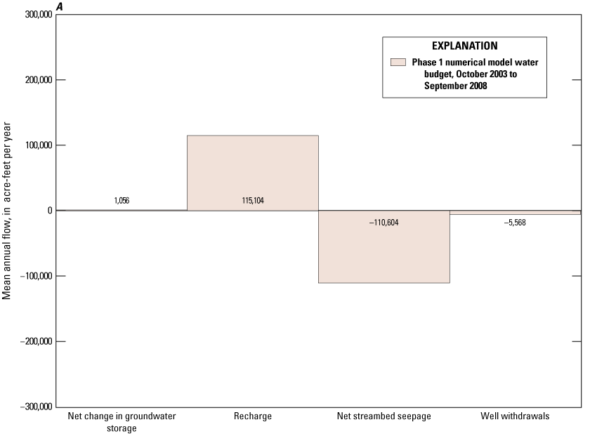
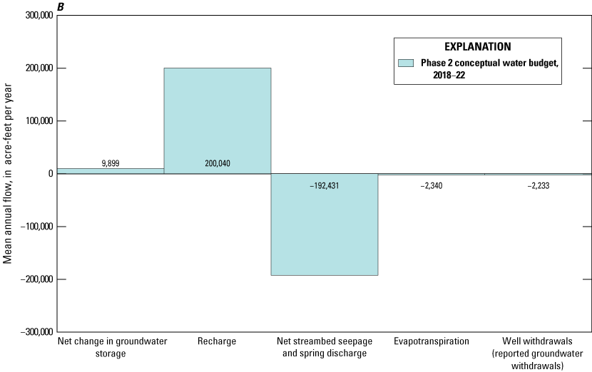
Water budgets for the eastern part of the Arbuckle-Simpson aquifer during A, Phase 1 numerical model period (October 2003 to September 2008) and B, Phase 2 conceptual model period (2018–22 calendar years), south-central Oklahoma.
Reported groundwater use (groundwater withdrawals) was averaged annually for the 2018–20 period. The net change in groundwater storage was calculated by analyzing the groundwater levels in the study area for Phase 2 (2019–23) (fig. 11); the average decline in groundwater levels in the eastern part of the Arbuckle-Simpson aquifer was determined as approximately 3 ft/yr. A specific yield of 0.01 was reported by Christenson and others (2011) as the average specific yield of the eastern part of the Arbuckle-Simpson aquifer. To calculate the net change in groundwater storage, the 3-ft/yr change in groundwater levels was multiplied by the specific yield of 0.01 and then multiplied by the aquifer area.
The two largest components of the water budget, recharge and net streambed seepage, were greater in Phase 2 than in Phase 1 by 74 percent and 74 percent, respectively. Evapotranspiration from the saturated zone was not individually accounted for in the numerical water budget for Phase 1. Groundwater withdrawals in Phase 2 decreased by 60 percent from Phase 1 groundwater withdrawals. Groundwater storage in the water budget consists of flow that is sourced from the storage in the aquifer; therefore, a positive mean annual flow for groundwater storage indicates flow to the groundwater flow system came from storage, which results in a decrease in the aquifer storage. The net change in groundwater storage increased by approximately 837 percent (8,843 acre-feet per year) from Phase 1 to Phase 2, indicating a decrease in aquifer storage (decline in groundwater levels) in the Arbuckle-Simpson aquifer from Phase 1 to Phase 2 (fig. 16; table 13).
Table 13.
Phase 2 conceptual water budget for the eastern part of the Arbuckle-Simpson aquifer, south-central Oklahoma (2018–22).[acre-ft/yr, acre-feet per year; --, not quantified; in/yr, inch per year; ft/yr, foot per year; OWRB, Oklahoma Water Resources Board; NWI, National Wetlands Inventory; PART, hydrograph-separation method for determining base flow; ET, evapotranspiration; SWB, Soil-Water-Balance (Westenbroek and others, 2010); GW, groundwater]
Overall, the water budget for the eastern part of the Arbuckle-Simpson aquifer during Phase 2 appears to include more groundwater inflow, more groundwater outflow, and more groundwater flow from storage (decreased aquifer storage) than during Phase 1. This is apparent from the increase in precipitation, recharge, streamflow, and base flow and the decrease in groundwater levels. However, discharge from springs both increased and decreased at sites measured during the historical period and Phase 2. Outflows, such as groundwater withdrawals, were smaller in Phase 2 compared to Phase 1.
Future Studies and Monitoring Data
To quantify water resources for a natural system and thus provide information that will help to address water resource management questions, the first step is to collect accurately measured water-quantity-related data. The scales (temporal and spatial) for which a water resource manager attempts to answer water management questions is the scale for which these quantity data should be measured. The time interval is an important consideration for data collection and will vary depending on whether the goal is to try to capture subdaily, daily, monthly, or annual effects on the water resources. In addition, the scale and scope of the data collected across a study area should be dependent on the scale of the questions being asked. This report contains compiled daily or subdaily measured quantities of precipitation, streamflow, springflow, and groundwater levels across the study area. However, reported groundwater withdrawals and water pumped from mine pits and discharges from producing mines presented in this report are compiled from self-reported or estimated quantities on monthly or annual timescales. Human activities that release water into these natural systems complicate analyses for hydrologists and water-resource managers when they are not measured. For example, stream augmentation that occurs from mines affects streamflow hydrographs and analysis of streamflow for determination of base flow (fig. 7). Additional analysis on quantifying these anthropogenic stream augmentations from natural discharges on hydrographs, obtaining discharge rates of releases to streams from the mines, or deploying a device that measures these discharges would be beneficial to future studies to fully analyze the effects of streamflow augmentation on streamflow (and potentially recharge to the aquifer). Future plans and studies by hydrologists and water resource managers to answer application-specific questions about the Arbuckle-Simpson aquifer could benefit from additional data collection, such as the installation of data collection sites for monitoring daily volumetric outflow (pumping and discharging) rates. The collection of daily volumetric outflow monitoring data could help to reduce the uncertainty in those data that were estimated in this report.
Summary
Based primarily on data collected between 2003 and 2008, a series of comprehensive hydrologic studies of the Arbuckle-Simpson aquifer in south-central Oklahoma was published between 2003 and 2011. For this report, “Phase 1” refers to an initial 2003–08 data collection period, although for some analyses, data collected prior to 2003 were used to inform model development. Results from Phase 1 provided information necessary to perform groundwater-flow model simulations that, in addition to characterizing groundwater resources in the study area, helped inform the Oklahoma Water Resources Board (OWRB) in their decisions regarding how much water could be withdrawn from the aquifer while maintaining flow to springs and streams. As part of the Phase 1 studies, an aquifer water budget was developed from a numerical model for the period 2003–08. Allocation of water from this aquifer was then established by the OWRB in 2013. Additional well-spacing rules were also established by the OWRB for sensitive sole source groundwater basins.
To determine how the water budget for the eastern part of the Arbuckle-Simpson aquifer has changed over time, recently collected hydrologic data (2018–23) were compared to data collected during 2003–08. The analysis of changes in the aquifer water budget from 2003–08 to 2018–23 could help resource managers better understand changes in the overall balance of water in storage and potential effects to streamflow, changes in groundwater levels, and the effects of different water uses in the aquifer area on available water in both the eastern part of the Arbuckle-Simpson aquifer and streams overlying the eastern part of the Arbuckle-Simpson aquifer. This report documents the results of a study done by the U.S. Geological Survey (USGS), in cooperation with the OWRB and the Oka’ Institute, to document recently collected (2018–23) hydrologic data and assess water-budget changes for the eastern part of the Arbuckle-Simpson aquifer.
The Arbuckle Mountains are composed of Proterozoic- and Cambrian-aged igneous and metamorphic rocks overlain by sedimentary rocks that are Cambrian to Late Pennsylvanian in age. The geology of the Arbuckle Mountains is characterized by both macro- and meso-scale deformations, consisting of folded structures, large fault displacements, uplifts, and karstic features developing in their carbonate sedimentary rocks. Sinkholes, caves, springs, and other characteristic karst features are present throughout the Arbuckle Mountains. Because all these features affect the flow and availability of groundwater in the study area, the geologic framework of the Arbuckle Mountains is considered when assessing groundwater in the Arbuckle-Simpson aquifer.
The Arbuckle Group is approximately 3,000 feet thick in most of the eastern part of the Arbuckle-Simpson aquifer study area but has been eroded away over parts of the Belton Anticline. The portion of the Arbuckle-Simpson aquifer contained in the Arbuckle Group is more productive than the portion contained in the Simpson Group because of its intercrystalline porosity and the numerous fractures, solution channels, and cavities it contains. The Simpson Group was deposited in the Middle to Late Ordovician and is the younger of the lithostratigraphic groups contained in the Arbuckle-Simpson aquifer. The Simpson Group is generally less than 1,000 feet thick in the eastern part of the Arbuckle-Simpson aquifer and is exposed at the surface in about one-third of the total aquifer area, typically along the edges of major anticlines and other structurally low areas.
The mean annual precipitation for the 1895–2022 period was 37.97 inches per year (in/yr) for the eastern part of the Arbuckle-Simpson aquifer that extends across four counties in Oklahoma's south-central climate division, Climate Division 8. The minimum temperature recorded was 16.4 degrees Fahrenheit in February 1899, and the maximum recorded temperature was 104.7 degrees Fahrenheit in August 2011, with an overall increase in temperature of 0.04 degree Fahrenheit per decade during the 1895–2022 period.
Seven new USGS streamgages that monitor discharge were installed on streams flowing across the eastern part of the Arbuckle-Simpson aquifer as a part of Phase 2; in addition, five streamgages in the study area were used to monitor streamflow during Phase 1 and were still operational at the start of Phase 2. Streamflow is lowest in the summer (June–August) and winter (December–February), likely because of lower precipitation rates compared to the spring (April–May) and fall (September–November), as well as higher evapotranspiration rates in the summer. Base-flow separation was completed for three streamgages where streamflow data were collected for both Phase 1 and Phase 2. Base flow increased from Phase 1 to Phase 2 at all three streamgages. However, the base-flow portion of streamflow decreased from Phase 1 to Phase 2 at two of the three streamgages analyzed.
One issue with attempting to compute the base-flow portion of streamflow is the influence of anthropogenic discharges upstream, such as stream augmentation from producing mines. These discharges affect streamflows measured and analyses of streamflows for interpretation of groundwater and surface-water interactions and base-flow analyses. The increases in the base-flow portion of streamflow and total streamflow during Phase 2 could be related to these upstream discharges.
Net gains and losses in streamflow along stream segments were quantified by using discrete discharge measurements made during base-flow conditions, commonly referred to as synoptic base-flow (seepage-run) measurements. To ensure base-flow conditions were being captured, with as little runoff as possible, streamflow discharge was measured during January 24–31, 2022, and February 28–March 1, 2023. The 2022 seepage measurements indicated net gaining stream reaches along portions of Rock Creek, Mill Creek, Pennington Creek, and the Blue River. Upstream reaches of the Blue River were net losing, indicating net seepage losses from the stream into the Arbuckle-Simpson aquifer. The upper reaches of Pennington Creek and Mill Creek had no flow. Delaware Creek and Little Blue Creek (tributary to the Blue River) had losing segments. The 2023 seepage measurements indicated that more stream segments were gaining than during the 2022 measurements on Mill Creek, Pennington Creek, Blue River, Little Blue Creek, and Delaware Creek. In addition, streamflows computed at USGS streamgages in the study area were generally greater during the period when the 2023 measurements were made than during the period when the 2022 measurements were made.
Discharge was continuously monitored at USGS streamgages at four major springs in the study area: Antelope Spring, unnamed Blue River spring, Byrds Mill Spring, and Sheep Creek Spring. Spring discharge was generally lower in summer and winter when there is typically less precipitation compared to fall and spring, and evaporation losses reach their annual peak in the summer, which also causes spring discharge to decrease relatively more than during other seasons. For all seasons, spring discharges were generally highest during the spring because seasonal precipitation amounts are highest and because evapotranspiration rates in the spring are relatively low compared to those in the summer. Continuous spring discharge hydrographs from the Antelope Spring gage, Byrds Mill Spring gage, and Sheep Creek Spring gage were analyzed for the highest discharge periods during 2015–16 to identify flow regimes of this karst aquifer. As indicated by the recession curves at the highest discharge periods, Antelope Spring exhibits more conduit flow than during the other periods of recession, followed by greater portions of mixed and diffuse flow. Discharge data from the Byrds Mill and Sheep Creek Spring gages indicate that these springs, near the upper levels of the formation, undergo relatively more diffuse flow periods than Antelope Spring.
Spring discharges were not measured and documented specifically for the Phase 1 studies, but historical spring discharges from the USGS National Water Information System database (1954–2017) were analyzed by the OWRB to identify which springs to include for the well-spacing rules for sensitive sole-source groundwater basins. Spring discharges for Phase 2 were measured during 2018–23 for comparison to historical spring discharges. Eleven of the 17 spring sites had a decrease in discharge from the historical period to Phase 2.
The continuous groundwater monitoring network that was established for Phase 2 consisted of 23 wells, with 18 wells completed in the Arbuckle Group and 5 wells completed in the Simpson Group. Groundwater-level data from Phase 1 were compared to those collected during Phase 2 at five wells, with the results indicating relatively unchanged mean groundwater levels. The periods of lowest groundwater levels typically occurred during the summer and winter months, and the troughs in the groundwater-level hydrographs were generally shallower during Phase 2 than during Phase 1. Water levels in the study area during the summer and winter, particularly in the Arbuckle Group, appear to be generally decreasing during the Phase 2 period. These declining water levels seem to have been caused by decreasing precipitation, but they could also have been caused by increased water use or evapotranspiration. Groundwater-level data from 57 groundwater wells in 2022 and 56 wells in 2023 were used to create two potentiometric-surface maps over the main area of the eastern part of the Arbuckle-Simpson aquifer. The largest differences in water-level altitudes between 2022 and 2023 were in an area of four wells east of Pennington Creek. Even with localized differences between the two maps, general patterns remained similar in 2022 and 2023. Potentiometric surfaces indicate that regional groundwater flow is toward the southeast, where streams and springs discharge at the aquifer boundary.
Two methods were used in this study to estimate recharge: a recession-curve displacement method, or RORA method, was used to estimate recharge in a watershed upstream from three selected streamgages, and the Soil-Water-Balance (SWB) code was used to model spatially distributed recharge rates across the aquifer. The mean annual estimated recharge determined by using the RORA program for the eastern part of the Arbuckle-Simpson aquifer was 16.5 in/yr (or 43 percent of the 37.97 inches of mean annual precipitation) during 2018–22. Phase 2 mean annual recharge determined by using the RORA program was greater than Phase 1 mean annual recharge. For the Blue River near Connerville gage, the mean annual recharge increased by 98 percent from Phase 1 to Phase 2. For the Pennington Creek near Reagan gage, the mean annual recharge increased by 33 percent from Phase 1 to Phase 2. The same issue mentioned for base-flow analysis of streamflow also affects recharge estimates obtained from the RORA program. Upstream anthropogenic streamflow augmentation from producing mines affects recharge estimates obtained from the RORA program by increasing the part of the hydrograph that is interpreted by the RORA program as recharge to the aquifer. The SWB code was run to estimate the amount and spatial distribution of daily groundwater recharge to the eastern part of the Arbuckle-Simpson aquifer only for 2019–22. The mean annual SWB-estimated recharge for the eastern part of the Arbuckle-Simpson aquifer was 4.85 in/yr (or 13 percent of the 7.97 inches of mean annual precipitation) for the 2019–22 period. The annual SWB-estimated recharge for the eastern part of the Arbuckle-Simpson aquifer was 7.2 inches for 2019, 5.9 inches for 2020, 2.6 inches for 2021, and 3.6 inches for 2022.
Nine different beneficial groundwater-use types are regulated by the OWRB for groundwater permits: (1) irrigation, (2) public supply, (3) industrial, (4) power, (5) mining, (6) commercial, (7) recreation, fish, and wildlife, (8) agricultural, and (9) other. Public supply was the most reported beneficial groundwater-use type during 1967–2020 for the eastern part of the Arbuckle-Simpson aquifer, with the aquifer providing water for municipalities within the study area. The mean annual reported groundwater use during 1967–2020 was 3,251 acre-feet.
Management plans and reports submitted to the OWRB by mines for monitoring and periodic reporting of groundwater disposition include a water budget for the mine that describes anticipated water moving into and out of the mine site as stream and groundwater inflows and outflows (includes augmentation outflows to streams and the groundwater system), pit water, precipitation runoff, and evaporation. These water volumes are used by the OWRB to estimate the consumptive use of pit water. Water volume data from these management plans and reports were compiled for 2019–22 and summarized in this report. The sum of the water withdrawn from mine pits, sum of stream augmentation, and sum of groundwater augmentation are also reported for each year for the eight mines for which compiled water-use data were available.
As part of the Phase 1 studies, the USGS developed an aquifer water budget from a numerical model for the October 2003 to September 2008 period. The Phase 2 water budget was summarized by using the data in this report for a conceptual water budget for the 2018–22 calendar years because as of the writing of this report, a numerical model had not yet been developed for Phase 2 that could be used to assess the water budget more accurately. Overall, the water budget for the eastern part of the Arbuckle-Simpson aquifer during Phase 2 appears to include more groundwater inflow, more groundwater outflow, and more groundwater flow from storage (decreased aquifer storage) than during Phase 1. This is apparent from the increase in precipitation, recharge, streamflow, and base flow and the decrease in groundwater levels. However, discharge from springs both increased and decreased at sites measured during the historical period and Phase 2. Outflows, such as groundwater withdrawals, were smaller in Phase 2 compared to Phase 1.
This report contains compiled daily or subdaily measured quantities of precipitation, streamflow, springflow, and groundwater levels across the study area. However, reported groundwater withdrawals and water pumped from mine pits and discharges from producing mines presented in this report are compiled from self-reported or estimated quantities on monthly or annual timescales. Human activities that release water into these natural systems complicate analyses for hydrologists and water-resource managers when they are not measured. Future plans and studies by hydrologists and water resource managers to answer application-specific questions about the Arbuckle-Simpson aquifer could benefit from additional data collection, such as the installation of data collection sites for monitoring daily volumetric outflow (pumping and discharging) rates. The collection of daily volumetric outflow monitoring data could help to reduce the uncertainty in those data that were estimated in this report.
References Cited
Barlow, P.M., Cunningham, W.L., Zhai, T., and Gray, M., 2015, U.S. Geological Survey Groundwater Toolbox, a graphical and mapping interface for analysis of hydrologic data (version 1.0)—User guide for estimation of base flow, runoff, and groundwater recharge from streamflow data: U.S. Geological Survey Techniques and Methods, book 3, chap. 10, 27 p., accessed June 5, 2023, at https://doi.org/10.3133/tm3B10.
Campbell, J.A., and Weber, J.L., 2006, Wells drilled to basement in Oklahoma: Oklahoma Geological Survey Special Publication 2006-1, 1 p., accessed December 11, 2023, at http://ogs.ou.edu/docs/specialpublications/SP2006-1P1.pdf.
Cates, S.W., 1989, Fault distribution in the Sulphur, Oklahoma area based on gravity, magnetic and structural data: Norman, Okla., University of Oklahoma, M.S. thesis, 106 p., accessed December 11, 2023, at https://shareok.org/handle/11244/51939.
Chase, B.F., Kolawole, F., Atekwana, E.A., Carpenter, B.M., Turko, M., Abdelsalam, M., and Finn, C., 2022, The 180-km-long Meers-Willow fault system in the Southern Oklahoma Aulacogen—A potential U.S. mid-continent seismic hazard: Geological Society of America Bulletin, v. 135, no. 3–4, p. 663–677, accessed December 11, 2023, at https://doi.org/10.1130/B36363.1.
Christenson, S., Hunt, A.G., and Parkhurst, D.L., 2009, Geochemical investigation of the Arbuckle-Simpson aquifer, south-central Oklahoma, 2004–06: U.S. Geological Survey Scientific Investigations Report 2009–5036, 51 p., accessed December 11, 2023, at https://doi.org/10.3133/sir20095036.
Christenson, S., Osborn, N.I., Neel, C.R., Faith, J.R., Blome, C.D., Puckette, J., and Pantea, M.P., 2011, Hydrogeology and simulation of groundwater flow in the Arbuckle-Simpson aquifer, south-central Oklahoma: U.S. Geological Survey Scientific Investigations Report 2011–5029, 104 p., accessed December 11, 2023, at https://doi.org/10.3133/sir20115029.
Cleveland, W.S., 1979, Robust locally weighted regression and smoothing scatterplots: Journal of the American Statistical Association, v. 74, no. 368, p. 829–836, accessed May 28, 2024, at https://doi.org/10.1080/01621459.1979.10481038.
Cunningham, W.L., and Schalk, C.W., comps., 2011, Groundwater technical procedures of the U.S. Geological Survey: U.S. Geological Survey Techniques and Methods, book 1, chap. A1, 151 p., accessed December 30, 2024, at https://doi.org/10.3133/tm1A1.
Denison, R.E., 1973, Basement rocks in the Arbuckle Mountains, in Ham, W.E., ed., Regional geology of the Arbuckle Mountains, Oklahoma: Oklahoma Geological Survey Special Publication 73–3, p. 43–46, accessed May 28, 2024, at http://ogs.ou.edu/docs/specialpublications/SP73-3.pdf.
Denison, R.E., 1995, Significance of air-photograph linears in the basement rocks of the Arbuckle Mountains, in Johnson, K.S., ed., Structural styles in the southern Midcontinent, 1992 Symposium: Oklahoma Geological Survey Circular 97, p. 119–131, accessed December 11, 2023, at http://ogs.ou.edu/docs/circulars/C97.pdf.
Denison, R.E., 1997, Contrasting sedimentation inside and outside the Southern Oklahoma aulacogen during the Middle and Late Ordovician, in Johnson, K.S., ed., Simpson and Viola Groups in the southern Midcontinent, 1994 Symposium: Oklahoma Geological Survey Circular 99, p. 39–47, accessed December 11, 2023, at http://ogs.ou.edu/docs/circulars/C99.pdf.
Donovan, R.N., 1991, The Arbuckle Group—An aide de memoire, in Johnson, K.S., ed., Arbuckle Group Core Workshop and Field Trip: Oklahoma Geological Survey Special Publication 91–3, p. 199–208, accessed December 11, 2023, at http://ogs.ou.edu/docs/specialpublications/SP91-3.pdf.
English, J.M., and Johnston, S.T., 2004, The Laramide orogeny—What were the driving forces?: International Geology Review, v. 46, p. 833–838, accessed January 10, 2025, at http://neotectonics.seismo.unr.edu/0_COURSES/Geo730-2020/EnglishLaramide2004.pdf.
Esri, 2024, ArcGIS for desktop help—Fill tool: Esri web page, accessed January 31, 2024, at https://desktop.arcgis.com/en/arcmap/10.7/tools/spatial-analyst-toolbox/fill.htm.
Fairchild, R.W., Hanson, R.L., and Davis, R.E., 1990, Hydrology of the Arbuckle Mountains area, south-central Oklahoma: Oklahoma Geological Survey Circular 91, 112 p., 2 pls., scale 1:100,000, accessed December 11, 2023, at http://ogs.ou.edu/docs/circulars/C91.pdf.
Faith, J.R., Blome, C.D., Pantea, M.P., Puckette, J.O., Halihan, T., Osborn, N., Christenson, S., and Pack, S., 2010, Three-dimensional geologic model of the Arbuckle–Simpson aquifer, south-central Oklahoma: U.S. Geological Survey Open-File Report 2010–1123, 29 p., accessed December 11, 2023, at https://doi.org/10.3133/ofr20101123.
Greenlee, D.D., 1987, Raster and vector processing for scanned linework: Photogrammetric Engineering and Remote Sensing, v. 53, no. 10, p. 1383–1387, accessed May 28, 2024, at https://www.asprs.org/wp-content/uploads/pers/1987journal/oct/1987_oct_1383-1387.pdf.
Halihan, T., Mouri, S., and Puckette, J., 2009a, Evaluation of fracture properties of the Arbuckle-Simpson aquifer—Final report submitted to the Oklahoma Water Resources Board: Oklahoma State University, School of Geology, 64 p., accessed May 28, 2024, at https://rest.owrb.ok.gov/studies/groundwater/arbuckle_simpson/pdf/2009_Reports/EvaluationFracturePropertiesArbuckleSimpson_Halihan.pdf.
Halihan, T., Puckette, J., Sample, M., and Riley, M., 2009b, Electrical resistivity imaging of the Arbuckle-Simpson aquifer—Final report submitted to the Oklahoma Water Resources Board: Stillwater, Okla., Oklahoma State University, School of Geology, 152 p., accessed May 28, 2024, at https://www.owrb.ok.gov/studies/groundwater/arbuckle_simpson/pdf/2009_Reports/ElectricResistivityImagingArbuckle_Halihan.pdf.
Ham, W.E., 1945, Geology and glass sand resources, central Arbuckle Mountains, Oklahoma: Oklahoma Geological Survey Bulletin 65, 103 p., accessed December 11, 2023, at http://ogs.ou.edu/docs/bulletins/B65.pdf.
Ham, W.E., 1973, Regional geology of the Arbuckle Mountains, Oklahoma: Oklahoma Geological Survey Special Publication 73–3, 61 p., accessed December 11, 2023, at http://ogs.ou.edu/docs/specialpublications/SP73-3.pdf.
Ham, W.E., Denison, R.E., and Merritt, C.A., 1964, Basement rocks and structural evolution of Southern Oklahoma: Oklahoma Geological Survey Bulletin 95, 302 p., 5 pls., accessed December 12, 2023, at http://ogs.ou.edu/docs/bulletins/B95.pdf.
Hargreaves, G.H., and Samani, Z.A., 1985, Reference crop evapotranspiration from temperature: Applied Engineering in Agriculture, v. 1, no. 2, p. 96–99, accessed December 12, 2023, at https://doi.org/10.13031/2013.26773.
Harlton, B.H., 1966, Relation of buried Tishomingo Uplift to Ardmore basin and Ouachita Mountains, southeastern Oklahoma: American Association of Petroleum Geologists Bulletin, v. 50, no. 7, p. 1365–1374, accessed December 12, 2023, at https://archives.datapages.com/data/bulletns/1965-67/images/pg/00500007/1350/13650.pdf.
Heran, W.D., Green, G.N., and Stoeser, D.B., 2003, A digital geologic map database for the State of Oklahoma: U.S. Geological Survey Open-File Report 03–247, accessed June 14, 2023, at https://pubs.usgs.gov/of/2003/ofr-03-247/.
Johnson, K.S., 1991, Geologic overview and economic importance of Late Cambrian and Ordovician rocks in Oklahoma, in Johnson, K.S., ed., Late Cambrian–Ordovician geology of the southern Midcontinent, 1989 Symposium: Oklahoma Geological Survey Circular 92, p. 3–14, accessed December 12, 2023, at http://ogs.ou.edu/docs/circulars/C92.pdf.
Johnson, K.S., Amsden, T.W., Denison, R.E., Dutton, S.P., Goldstein, A.G., Rascoe, B., Sutherland, P.K., and Thompson, D.M., 1989, Geology of the southern Midcontinent: Oklahoma Geological Survey Special Publication 89–2, 53 p., accessed December 12, 2023, at http://ogs.ou.edu/docs/specialpublications/SP89-2.pdf.
Kennedy, B., Young, R.A., and Russian, C., 2009, Seismic evidence of faulting at three different geologic scales in the Arbuckle‐Simpson aquifer, Oklahoma, in Butler, D.K., ed., Symposium on the Application of Geophysics to Engineering and Environmental Problems Proceedings: Environmental & Engineering Geophysical Society, p. 281–290, accessed December 12, 2023, at https://doi.org/10.4133/1.3176705.
Levesque, V.A., and Oberg, K.A., 2012, Computing discharge using the index velocity method: U.S. Geological Survey Techniques and Methods, book 3, chap. A23, 148 p., accessed December 23, 2024, at https://doi.org/10.3133/tm3A23.
Lynch, M., and Al-Shaieb, Z., 1991, Evidence of paleokarst phenomena and burial diagenesis in the Ordovician Arbuckle Group of Oklahoma, in Johnson, K.S., ed., Late Cambrian–Ordovician geology of the southern Midcontinent, 1989 Symposium: Oklahoma Geological Survey Circular 92, p. 42–60, accessed December 12, 2023, at http://ogs.ou.edu/docs/circulars/C92.pdf.
Mashburn, S.L., Kirby, E.A., and Wagner, D.L., 2025, Soil-Water-Balance model and data for Phase 1 (2003–08) and Phase 2 (2018–23) hydrologic and water-budget analyses of the eastern part of the Arbuckle-Simpson aquifer, south-central Oklahoma, 2019–22: U.S. Geological Survey data release, https://doi.org/10.5066/P14UXYVV.
Multi-Resolution Land Characteristics Consortium, 2024, National Land Cover Database (NLCD) 2021: U.S. Geological Survey database, accessed January 31, 2024, at https://www.mrlc.gov/data.
National Centers for Environmental Information [NCEI], 2023, Climate at a glance—National time series: National Oceanic and Atmospheric Administration database, accessed August 25, 2023, at https://www.ncei.noaa.gov/access/monitoring/climate-at-a-glance/national/time-series.
National Ecological Observatory Network [NEON], 2023, Explore data products: National Ecological Observatory Network web page, accessed August 7, 2023, at https://data.neonscience.org/data-products/explore.
Oklahoma Climatological Survey, 2023, Climate of Oklahoma: Oklahoma Climatological Survey web page, accessed August 10, 2023, at https://climate.ok.gov/index.php/site/page/climate_of_oklahoma.
Oklahoma Mesonet, 2023, Daily data retrieval: Oklahoma Mesonet database, accessed August 10, 2023, at https://www.mesonet.org/past-data/mesonet-resources/daily-data-retrieval.
Oklahoma State Legislature, 2023a, Appropriation and use of stream water, chap. 20 of Oklahoma Water Resources Board: Oklahoma Statutes, title 785, accessed November 15, 2023, at https://rules.ok.gov/codes.
Oklahoma State Legislature, 2023b, Taking and use of groundwater, chap. 30 of Oklahoma Water Resources Board: Oklahoma Statutes, title 785, accessed November 15, 2023, at https://rules.ok.gov/codes.
Oklahoma State Legislature, 2023c, Well spacing, chap. 30, subchapter 3, section 6 of Oklahoma Water Resources Board: Oklahoma Statutes, title 785, accessed November 15, 2023, at https://rules.ok.gov/code.
Oklahoma State Legislature, 2023d, Annual reports of water use, chap. 30, subchapter 5, section 9 of Oklahoma Water Resources Board: Oklahoma Statutes, title 785, accessed November 15, 2023, at https://rules.ok.gov/code.
Oklahoma State Legislature, 2023e, Water trapped in producing mines, chap. 30, subchapter 15 of Oklahoma Water Resources Board: Oklahoma Statutes, title 785, accessed November 15, 2023, at https://rules.ok.gov/code.
Oklahoma Water Resources Board [OWRB], 2003, The Arbuckle-Simpson hydrology study—Management and protection of an Oklahoma water resource: Oklahoma Water Resources Board Fact Sheet, 4 p., accessed November 16, 2023, at https://oklahoma.gov/content/dam/ok/en/owrb/documents/science-and-research/hydrologic-investigations/arbuckle-simpson-fact-sheet.pdf.
Oklahoma Water Resources Board [OWRB], 2007, The Arbuckle-Simpson hydrology study newsletter—March 2007: Oklahoma Water Resources Board, 4 p., accessed June 24, 2024, at https://www.owrb.ok.gov/studies/groundwater/arbuckle_simpson/pdf/arbuckle_newsletter_0307.pdf.
Oklahoma Water Resources Board [OWRB], 2009, The Arbuckle-Simpson hydrology study—Final report to the U.S. Bureau of Reclamation, 42 p., accessed December 20, 2024, at https://www.owrb.ok.gov/studies/groundwater/arbuckle_simpson/pdf/09_report_burec.pdf.
Oklahoma Water Resources Board [OWRB], 2023, Oklahoma groundwater resources—Groundwater basins with final maximum annual yield determination: Oklahoma Water Resources Board, 1 sheet, accessed December 15, 2023, at https://oklahoma.gov/content/dam/ok/en/owrb/documents/maps-and-data/printable-maps/GW_Groundwater_Basins_with_MAY.pdf.
Oklahoma Water Resources Board [OWRB], 2024a, GIS data—Aquifers: Oklahoma Water Resources Board database, accessed January 31, 2024, at https://oklahoma.gov/owrb/data-and-maps/gis-data.html.
Oklahoma Water Resources Board [OWRB], 2024b, Pit water monitoring reports: Oklahoma Water Resources Board web page, accessed February 6, 2024, at https://oklahoma.gov/owrb/water-permitting/pit-water-monitoring-reports.html.
Otero, C.L., 2007, Geologic, hydrologic, and geochemical identification of flow paths in the Edwards aquifer, northeastern Bexar and southern Comal Counties, Texas: U.S. Geological Survey Scientific Investigations Report 2007–5285, 48 p., accessed October 12, 2023, at https://doi.org/10.3133/sir20075285.
Perry, W., Jr., 1989, Tectonic evolution of the Anadarko basin region, Oklahoma: U.S. Geological Survey Bulletin 1866–A, 19 p., accessed June 24, 2024, at https://doi.org/10.3133/b1866A.
Puckette, J., 2009, Analysis of bit cuttings, wire-line logs and flow tests from a deep test well in the Arbuckle-Simpson aquifer, Johnston County, Oklahoma—Final report submitted to the Oklahoma Water Resources Board: Stillwater, Okla., Oklahoma State University, School of Geology, 30 p., accessed June 24, 2024, at https://www.owrb.ok.gov/studies/groundwater/arbuckle_simpson/pdf/2009_Reports/AnalysisBitCuttingsWireLineLogsFlowTestsDeepTestWellArbuckle_Puckette.pd f.
Puckette, J., Halihan, T., and Faith, J., 2009, Characterization of the Arbuckle-Simpson aquifer—Final report submitted to the Oklahoma Water Resources Board: Stillwater, Okla., Oklahoma State University, School of Geology, 53 p., accessed June 24, 2024, at https://www.owrb.ok.gov/studies/groundwater/arbuckle_simpson/pdf/2009_reports/characterization_puckette/2009_puckette%20et%20al_characterization%20of% 20the%20arbuckle%20simpson.pdf.
Rahi, K., and Halihan, T., 2009, Estimating selected hydraulic parameters of the Arbuckle-Simpson aquifer from the analysis of naturally-induced stresses—Final report submitted to the Oklahoma Water Resources Board: Stillwater, Okla., Oklahoma State University, School of Geology, 48 p., accessed June 25, 2024, at https://www.owrb.ok.gov/studies/groundwater/arbuckle_simpson/pdf/2009_Reports/Hydraulic_RahiHalihan/EstimatingHydraulicParametersAnalysisNaturallyIndu cedStressesArbuckle_RahiHallihan.pdf.
Rahi, K., and Halihan, T., 2012, Identifying aquifer type in fractured rock aquifers using harmonic analysis: Groundwater, v. 51, no. 1, p. 76–82, accessed June 25, 2024, at https://doi.org/10.1111/j.1745-6584.2012.00925.x.
Ramachandran, K., Tapp, B., Rigsby, T., and Lewallen, E., 2012, Imaging of fault and fracture controls in the Arbuckle-Simpson aquifer, southern Oklahoma, USA, through electrical resistivity sounding and tomography methods: International Journal of Geophysics, v. 2012, 10 p., accessed June 25, 2024, at https://doi.org/10.1155/2012/184836.
Rantz, S.E., and others, 1982, Measurement and computation of streamflow—Volume 1. Measurement of stage and discharge: U.S. Geological Survey Water-Supply Paper 2175, 284 p., accessed December 23, 2024, at https://doi.org/10.3133/wsp2175.
Riley, M.E., 2004, Investigation of fault properties using electrical resistivity imaging: Stillwater, Okla., Oklahoma State University, M.S. thesis, 104 p., accessed June 25, 2024, at http://hdl.handle.net/20.500.14446/8049.
Rogers, I.M.J., Smith, S.J., Gammill, N.C., Gillard, N.J., Lockmiller, K.A., Fetkovich, E.J., Correll, J.S., and Hussey, S.P., 2023, Hydrogeology and simulated groundwater availability in reaches 3 and 4 of the Washita River aquifer, southern Oklahoma, 1980–2017: U.S. Geological Survey Scientific Investigations Report 2023–5072, 83 p., accessed January 1, 2024, at https://doi.org/10.3133/sir20235072.
Rorabaugh, M.I., 1964, Estimating changes in bank storage and ground-water contribution to streamflow: International Association of Scientific Hydrology, publication 63, p. 432–441, accessed June 25, 2024, at https://iahs.info/uploads/dms/063044.pdf.
Rutledge, A.T., 1998, Computer programs for describing the recession of ground-water discharge and for estimating mean ground-water recharge and discharge from streamflow records—Update: U.S. Geological Survey Water-Resources Investigations Report 98–4148, 43 p., accessed June 25, 2024, at https://doi.org/10.3133/wri984148.
Sample, M.S., 2008, Characterization of the epikarst over the Hunton Anticline, Arbuckle-Simpson aquifer, Oklahoma: Stillwater, Okla., Oklahoma State University, M.S. thesis, 220 p., accessed June 25, 2024, at http://hdl.handle.net/20.500.14446/8052.
Sauer, V.B., and Turnipseed, D.P., 2010, Stage measurement at gaging stations: U.S. Geological Survey Techniques and Methods book 3, chap. A7, 45 p., accessed December 23, 2024, at https://doi.org/10.3133/tm3A7.
Scheirer, D.S., and Hosford Scheirer, A., 2006, Gravity investigations of the Chickasaw National Recreation Area, south-central Oklahoma: U.S. Geological Survey Open-File Report 2006–1083, 40 p., accessed December 12, 2023, at https://pubs.usgs.gov/of/2006/1083/.
Seilheimer, T.S., and Fisher, W.L., 2008, Instream flow assessment of streams draining the Arbuckle-Simpson aquifer—Final report submitted to the Oklahoma Water Resources Board: Stillwater, Okla., Oklahoma State University, 49 p., accessed December 12, 2023, at https://www.owrb.ok.gov/studies/groundwater/arbuckle_simpson/pdf/Arbuckle-SimpsonInstreamFlow.pdf.
Sharp, J.M., Jr., 2024, A glossary of hydrogeology: Guelph, Ontario, Canada, The Groundwater Project, 211 p., accessed September 9, 2024, at https://doi.org/10.21083/978-1-77470-079-2.
Smith, D.V., Deszcz-Pan, M., and Smith, B.D., 2009, Depth section imaging for portions of an airborne geophysical survey of the Hunton Anticline, south-central Oklahoma: Final administrative report to the Oklahoma Water Resources Board in fulfillment of the cooperative agreement #08C7OK002032407, 38 p., accessed December 12, 2023, at https://www.owrb.ok.gov/studies/groundwater/arbuckle_simpson/pdf/2009_Reports/DepthSectionImagingAirborneGeophysicalSurveyHuntonAnticline_SmithDeszczP anSmith.pdf.
Smith, S.J., Ellis, J.H., Paizis, N.C., Becker, C.J., Wagner, D.L., Correll, J.S., and Hernandez, R.J., 2021, Hydrogeology and model-simulated groundwater availability in the Salt Fork Red River aquifer, southwestern Oklahoma, 1980–2015: U.S. Geological Survey Scientific Investigations Report 2021–5003, 85 p., accessed January 1, 2024, at https://doi.org/10.3133/sir20215003.
Tarhule, A., 2009, Hydroclimatic reconstruction of the Arbuckle-Simpson aquifer using tree rings—Final report submitted to the Oklahoma Water Resources Board: University of Oklahoma, Department of Geography, 72 p., accessed December 12, 2023, at https://oklahoma.gov/content/dam/ok/en/owrb/documents/science-and-research/hydrologic-investigations/arbuckle-simpson-tree-ring-study.pdf.
Thornton, M.M., Shrestha, R., Wei, Y., Thornton, P.E., Kao, S-C., and Wilson, B.E., 2024, Daymet—Daily surface weather data on a 1-km grid for North America, version 4 R1: Oak Ridge National Laboratory Distributed Active Archive Center (ORNL DAAC) for Biogeochemical Dynamics digital data, accessed January 31, 2024, at https://doi.org/10.3334/ORNLDAAC/2129.
Turnipseed, D.P., and Sauer, V.B., 2010, Discharge measurements at gaging stations: U.S. Geological Survey Techniques and Methods, book 3, chap. A8, 87 p., accessed January 20, 2024, at https://doi.org/10.3133/tm3A8.
U.S. Board on Geographic Names, 2024, Domestic names: U.S. Geological Survey web page, accessed June 18, 2024, at https://www.usgs.gov/us-board-on-geographic-names/domestic-names.
U.S. Department of Agriculture, 2024, Gridded Soil Survey Geographic (gSSURGO) database for the conterminous United States: U.S. Department of Agriculture, Natural Resources Conservation Service, accessed June 24, 2024, at https://gdg.sc.egov.usda.gov/GDGHome_DirectDownLoad.aspx.
U.S. Environmental Protection Agency [EPA], 1989, Arbuckle-Simpson aquifer of south central Oklahoma sole source aquifer—Final determination: Federal Register, v. 54, no. 184, p. 39230–39232, accessed December 5, 2024, at https://archive.org/details/sim_federal-register-find_1989-09-25_54_184/page/39230/mode/2up.
U.S. Environmental Protection Agency [EPA], 2024a, Sole source aquifers for drinking water, accessed August 19, 2024, at https://www.epa.gov/dwssa/overview-drinking-water-sole-source-aquifer-program.
U.S. Environmental Protection Agency [EPA], 2024b, Integrated Compliance Information System (ICIS)—National Pollutant Discharge Elimination System (NPDES) Permit Limit and Discharge Monitoring Report (DMR) datasets: U.S. Environmental Protection Agency database, accessed January 15, 2024, at https://echo.epa.gov/tools/data-downloads/icis-npdes-dmr-and-limit-data-set.
U.S. Fish and Wildlife Service, 2024, National Wetland Inventory, wetlands dataset: U.S. Fish and Wildlife Service web page, accessed June 24, 2024, at https://www.fws.gov/program/national-wetlands-inventory/metadata.
U.S. Geological Survey [USGS], 2015, National Elevation Dataset (NED) 1/3 arc-second DEM: U.S. Geological Survey database, accessed September 21, 2015, at https://apps.nationalmap.gov/downloader/#/.
U.S. Geological Survey [USGS], 2023, USGS National Hydrography Dataset: U.S. Geological Survey database, accessed December 2024, at https://www.usgs.gov/national-hydrography/national-hydrography-dataset.
U.S. Geological Survey [USGS], 2024a, USGS water data for the Nation: U.S. Geological Survey National Water Information System database, accessed January 2024, at https://doi.org/10.5066/F7P55KJN. [Oklahoma water data directly accessible at https://waterdata.usgs.gov/ok/nwis.]
U.S. Geological Survey [USGS], 2024b, National geologic map database (Geolex): U.S. Geological Survey database, accessed April 15, 2024, at https://ngmdb.usgs.gov/Geolex/search.
Vieux, B.E., and Moreno, M.A., 2008, Arbuckle-Simpson hydrology study—Distributed water resources assessment—Final report submitted to the Oklahoma Water Resources Board: Norman, Okla., University of Oklahoma, School of Civil Engineering and Environmental Science, 44 p., 11 app., accessed June 24, 2024, at https://www.owrb.ok.gov/studies/groundwater/arbuckle_simpson/pdf/2009_Reports/DistributedWaterResourcesAssessmentArbuckle_VieuxMorenoOWRB.pdf.
Westenbroek, S.M., Kelson, V.A., Dripps, W.R., Hunt, R.J., and Bradbury, K.R., 2010, SWB—A modified Thornthwaite-Mather Soil-Water-Balance code for estimating groundwater recharge: U.S. Geological Survey Techniques and Methods, book 6, chap. A31, 60 p., accessed January 15, 2024, at https://doi.org/10.3133/tm6A31.
White, W.N., 1932, A method of estimating ground-water supplies based on discharge by plants and evaporation from soil—Results of investigations in Escalante Valley, Utah: U.S. Geological Survey Water Supply Paper 659–A, 105 p., accessed August 20, 2024, at https://doi.org/10.3133/wsp659A.
Winter, T.C., Harvey, J.W., Franke, O.L., and Alley, W.M., 1998, Ground water and surface water—A single resource: U.S. Geological Survey Circular 1139, accessed May 31, 2024, at https://doi.org/10.3133/cir1139.
Young, R.A., Kennedy, B., and Russian, C., 2009, Analysis of seismic reflection data from the Hunton Anticline—Final report to the Oklahoma Water Resources Board: Oklahoma Water Resources Board, 13 p., accessed June 24, 2024, at https://www.owrb.ok.gov/studies/groundwater/arbuckle_simpson/pdf/2009_Reports/AnalysisSeismicReflectionDataHuntonAnticline_Young.pdf.
Appendix 1. Spring Discharge Measured in the Arbuckle-Simpson Aquifer
Table 1–1.
Springs with discharge greater than 50 gallons per minute based on historical data available in USGS NWIS database (USGS, 2024a), with springs having discharge greater than 500 gallons per minute that emanate from the Arbuckle-Simpson aquifer designated, a sensitive sole source groundwater basin, that are included in the well-spacing provisions established by the OWRB (Oklahoma State Legislature, 2023c).[USGS, U.S. Geological Survey; NWIS, USGS National Water Information System database; >, greater than; gal/min, gallons per minute. Springs listed are for the entire Arbuckle-Simpson aquifer across the western, central, and eastern parts]
Table 1–2.
Additional springs documented and discharge measured for Phase 2 (2018–23), south-central Oklahoma.[USGS, U.S. Geological Survey; ft3/s, cubic foot per second. Dates are in year-month-day format. Measurement ratings: excellent, discharge was within 2 percent of actual discharge; good, measured discharge within 5 percent of the actual discharge; fair, measured discharge within 10 percent of the actual discharge; poor and unspecified, measured discharge assumed to be within 8 percent of actual flow (Turnipseed and Sauer, 2010)]
| USGS station number (USGS, 2024a) | Latitude, in decimal degrees | Longitude, in decimal degrees | Date measured | Discharge, in ft3/s | Measurement rating | Spring short name |
|---|---|---|---|---|---|---|
| 342216096314001 | 34.379694 | −96.526972 | 2018-03-23 | 0.19 | Poor | Viola Spring |
| 342216096314001 | 34.379694 | −96.526972 | 2018-06-14 | 0.28 | Good | Viola Spring |
| 342233096444501 | 34.375333 | −96.746972 | 2018-04-20 | 0.17 | Fair | Caldwell Spring |
| 342233096444501 | 34.375333 | −96.746972 | 2018-06-13 | 0.02 | Poor | Caldwell Spring |
| 342254096425501 | 34.382389 | −96.715389 | 2018-03-26 | 0.35 | Poor | Spring Creek Spring |
| 342254096425501 | 34.382389 | −96.715389 | 2018-06-14 | 1.49 | Fair | Spring Creek Spring |
| 342254096425501 | 34.382389 | −96.715389 | 2022-09-12 | 7.98 | Good | Spring Creek Spring |
| 342335096462501 | 34.392861 | −96.774 | 2018-04-20 | 1.03 | Fair | Trent Spring |
| 342335096462501 | 34.392861 | −96.774 | 2018-06-13 | 0.35 | Fair | Trent Spring |
| 342342096464801 | 34.394889 | −96.781056 | 2018-04-20 | 0.34 | Fair | Gray Spring |
| 342342096464801 | 34.394889 | −96.781056 | 2018-06-28 | 0.26 | Poor | Gray Spring |
| 342414096364701 | 34.404056 | −96.613278 | 2018-03-23 | 0.42 | Fair | Diamond Spring |
| 342414096364701 | 34.404056 | −96.613278 | 2018-06-13 | 0.53 | Fair | Diamond Spring |
| 342511097064501 | 34.419667 | −97.111917 | 2018-03-22 | 1.39 | Poor | Devils Bathtub Spring |
| 342511097064501 | 34.419667 | −97.111917 | 2018-06-12 | 1.17 | Fair | Devils Bathtub Spring |
| 342518097064501 | 34.421917 | −97.112778 | 2018-03-21 | 0.506 | Fair | unnamed |
| 342522097101201 | 34.422778 | −97.170083 | 2018-03-21 | 0.0033 | Fair | unnamed |
| 342524097084701 | 34.423194 | −97.1465 | 2018-06-12 | 0.05 | Fair | unnamed |
| 342524097084701 | 34.423194 | −97.1465 | 2018-03-21 | 0.13 | Fair | unnamed |
| 342533097085401 | 34.425806 | −97.14825 | 2018-03-21 | 0.0222 | Fair | unnamed |
| 342533097085401 | 34.425806 | −97.14825 | 2018-06-12 | 0.019 | Fair | unnamed |
| 342614097114001 | 34.437333 | −97.194528 | 2018-06-12 | 0.09 | Fair | unnamed |
| 342614097114001 | 34.437333 | −97.194528 | 2018-03-21 | 0.21 | Poor | unnamed |
| 342718096380401 | 34.454972 | −96.634444 | 2018-06-13 | 0.91 | Fair | Anderson Spring |
| 342718096380401 | 34.454972 | −96.634444 | 2018-03-26 | 0.95 | Fair | Anderson Spring |
| 342718096380401 | 34.454972 | −96.634444 | 2022-09-13 | 0.56 | Fair | Anderson Spring |
| 342718096380401 | 34.454972 | −96.634444 | 2023-09-19 | 0.54 | Fair | Anderson Spring |
| 343007096581601 | 34.502 | −96.9712 | 2018-04-03 | 0.19 | Fair | unnamed |
| 343007096581601 | 34.502 | −96.9712 | 2018-06-12 | 0.11 | Fair | unnamed |
| 343012096581301 | 34.5028 | −96.9702 | 2018-03-22 | 0.0294 | Fair | unnamed |
| 343012096581301 | 34.5028 | −96.9702 | 2018-06-12 | 0.031 | Fair | unnamed |
| 343114096353101 | 34.5205 | −96.607806 | 2018-03-26 | 0.01 | Poor | Cave Spring |
| 343241096360201 | 34.54475 | −96.600833 | 2018-03-23 | 0.49 | Fair | Canyon Spring |
| 343241096360201 | 34.54475 | −96.600833 | 2018-06-13 | 0.60 | Fair | Canyon Spring |
| 343418096384201 | 34.57175 | −96.645083 | 2018-03-23 | 2.14 | Fair | unnamed |
| 343418096384201 | 34.57175 | −96.645083 | 2018-06-14 | 1.89 | Good | unnamed |
| 343422096385101 | 34.572778 | −96.6475 | 2018-03-23 | 3.43 | Good | Sheep Creek Spring |
| 343422096385101 | 34.572778 | −96.6475 | 2018-06-07 | 3.55 | Fair | Sheep Creek Spring |
| 342722096395501 | 34.456314 | −96.665522 | 2023-08-31 | 3.47 | Good | unnamed |
| 342722096395501 | 34.456314 | −96.665522 | 2023-09-19 | 3.06 | Fair | unnamed |
| 342723096395701 | 34.456464 | −96.666072 | 2023-08-31 | 2.77 | Fair | unnamed |
| 342723096395801 | 34.456433 | −96.666183 | 2023-08-31 | 1.52 | Fair | unnamed |
| 342247096425101 | 34.379861 | −96.714253 | 2023-09-19 | 5.10 | Good | unnamed |
| 342725096400701 | 34.457069 | −96.668692 | 2023-08-31 | 1.46 | Fair | unnamed |
| 342725096400701 | 34.457069 | −96.668692 | 2023-09-19 | 2.06 | Fair | unnamed |
| 342725096400801 | 34.4571 | −96.669119 | 2023-09-01 | 4.34 | Fair | unnamed |
| 342725096400801 | 34.4571 | −96.669119 | 2023-09-19 | 3.26 | Good | unnamed |
| 342726096395501 | 34.457422 | −96.665547 | 2023-09-01 | 0.95 | Poor | unnamed |
| 342726096395501 | 34.457422 | −96.665547 | 2023-09-19 | 1.11 | Poor | unnamed |
| 342726096400602 | 34.457344 | −96.668511 | 2023-08-31 | 0.06 | Poor | unnamed |
| 342726096400602 | 34.457344 | −96.668511 | 2023-09-19 | 0.04 | Poor | unnamed |
| 342726096400902 | 34.457306 | −96.669325 | 2019-09-19 | 3.13 | Fair | unnamed |
| 342726096400902 | 34.457306 | −96.669325 | 2023-09-28 | 3.32 | Fair | unnamed |
| 342726096400903 | 34.457253 | −96.669231 | 2019-09-19 | 3.13 | Good | unnamed |
| 342726096400903 | 34.457253 | −96.669231 | 2023-09-01 | 2.86 | Good | unnamed |
| 342726096401001 | 34.457325 | −96.669522 | 2023-09-01 | 0.07 | Poor | unnamed |
| 342726096401001 | 34.457325 | −96.669522 | 2023-09-19 | 0.14 | Poor | unnamed |
| 342911096373701 | 34.486481 | −96.627227 | 2022-09-12 | 1.48 | Poor | Willis Spring |
| 342911096373701 | 34.486481 | −96.627227 | 2023-09-19 | 1.91 | Poor | Willis Spring |
Conversion Factors
U.S. customary units to International System of Units
Temperature in degrees Fahrenheit (°F) may be converted to degrees Celsius (°C) as follows:
°C = (°F – 32) / 1.8.
Datums
Vertical coordinate information is referenced to the North American Vertical Datum of 1988 (NAVD 88).
Horizontal coordinate information is referenced to the North American Datum of 1983 (NAD 83).
Altitude, as used in this report, refers to distance above the vertical datum.
Abbreviations
bls
below land surface
DEM
digital elevation model
EPA
U.S. Environmental Protection Agency
NCEI
National Centers for Environmental Information
NPDES
National Pollutant Discharge Elimination System
NWIS
National Water Information System
OWRB
Oklahoma Water Resources Board
SWB
Soil-Water-Balance code
USGS
U.S. Geological Survey
For more information about this publication, contact
Director, Oklahoma-Texas Water Science Center
U.S. Geological Survey
1505 Ferguson Lane
Austin, TX 78754–4501
For additional information, visit
https://www.usgs.gov/centers/ot-water
Publishing support provided by
Lafayette Publishing Service Center
Disclaimers
Any use of trade, firm, or product names is for descriptive purposes only and does not imply endorsement by the U.S. Government.
Although this information product, for the most part, is in the public domain, it also may contain copyrighted materials as noted in the text. Permission to reproduce copyrighted items must be secured from the copyright owner.
Suggested Citation
Mashburn, S.L., Fetkovich, E.J., Lockmiller, H.A., Codner, C., Kirby, E.A., Dale, I.A., and Baciocco, C.A., 2025, Comparison of hydrologic data and water budgets between 2003–08 and 2018–23 for the eastern part of the Arbuckle-Simpson aquifer, south-central Oklahoma: U.S. Geological Survey Scientific Investigations Report 2025–5011, 61 p., https://doi.org/10.3133/sir20255011.
ISSN: 2328-0328 (online)
Study Area
| Publication type | Report |
|---|---|
| Publication Subtype | USGS Numbered Series |
| Title | Comparison of hydrologic data and water budgets between 2003–08 and 2018–23 for the eastern part of the Arbuckle-Simpson aquifer, south-central Oklahoma |
| Series title | Scientific Investigations Report |
| Series number | 2025-5011 |
| DOI | 10.3133/sir20255011 |
| Publication Date | March 14, 2025 |
| Year Published | 2025 |
| Language | English |
| Publisher | U.S. Geological Survey |
| Publisher location | Reston, VA |
| Contributing office(s) | Oklahoma-Texas Water Science Center |
| Description | Report: x, 61 p.; Data Release |
| Country | United States |
| State | Oklahoma |
| Other Geospatial | eastern part of the Arbuckle-Simpson Aquifer |
| Online Only (Y/N) | Y |