Figure 2.  Map showing tracklines of geophysical data collected by USGS (red and green lines) and NOAA (purple lines). USGS, U.S. Geological Survey; NOAA, National Oceanic and Atmospheric Administration. Click on figure for larger image.

Figure 3.  Photographs of research vessels used for mapping surveys in this project. A, RV Megan T. Miller; B, RV Rafael; C, RV Connecticut; D, RV Thomas Jefferson. Click on figure for larger image.

Figure 4.  Map showing shaded-relief topography of seafloor in study area. Coloring and bathymetric contours represent depths in meters, relative to the Mean Lower Low Water (MLLW) datum. Click on figure for larger image.

Figure 5.  Map showing sampling sites over acoustic-backscatter intensity in the study area.  Backscatter intensity is an acoustic measure of the hardness and roughness of the seafloor.  In general, higher values (light tones) represent rock, boulders, cobbles, gravel, and coarse sand.  Lower values (dark tones) generally represent fine sand and muddy sediment.  Tonal variations may occur across track in the sidescan-sonar data and between survey days in the multibeam echosounder data. Click on figure for larger image.

Figure 6.  Photograph of the SEABed Observation and Sampling System (SEABOSS), which was used to collect photographic data and sediment samples. Click on figure for larger image.

• Bathymetry

• Acoustic Backscatter

• Seismic-Reflection Profiling

  • Seismic-Reflection Data Acquisition 06012
  • Seismic-Reflection Data Acquisition 07001

• Ground Validation

  • Surficial Sediment Samples and Grain-Size Analyses
  • Photography and Video

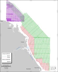
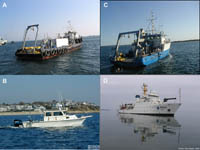
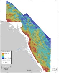
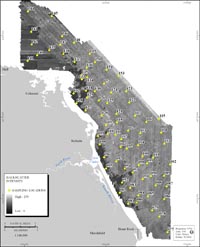
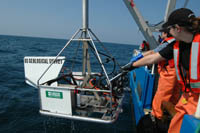
Bathymetry

Bathymetric data were acquired by the USGS using a Systems Engineering & Assessment Ltd (SEA) SwathPlus 234-kilohertz (kHz) interferometric sonar system at a ping rate of 0.25 seconds (s). During field activity 06012, the transducers were mounted on a rigid pole on the starboard side of the RV Megan T. Miller (fig. 3), about 2.6 m below the waterline. A TSS Ltd. Dynamic Motion Sensor (DMS) 2-05 motion reference unit was mounted directly above the sonar transducers and continuously measured vertical displacement (heave) and attitude (pitch and roll) of the vessel during acquisition.  During USGS field activity 07001, the transducers were mounted on a rigid pole on the bow of the RV Rafael, about 0.5 m below the waterline.  A CodaOctopus F-180 inertial-motion unit, mounted directly above the transducers, measured vertical displacement and attitude of the vessel during acquisition. Sound-velocity profiles were collected approximately every 2 hours using a hand-casted Applied MicroSystems SV Plus sound velocimeter.  Survey lines were run at an average speed of 5 knots and were spaced 100 m apart to obtain overlapping swaths of data and full coverage of the seafloor.  Navigation was based on a Real-Time Kinematic Global Positioning System (RTK-GPS).  The RTK-corrected GPS signal was sent to the ship from a base station established by the USGS on land.  Soundings were referenced to MLLW using orthometric to chart datum offsets obtained from NOAA Tidal Station #8446009 at Brant Rock Harbor, MA. SEA SwathPlus acquisition software and the Computer Aided Resource Information System (CARIS) Hydrographic Information Processing System (HIPS version 6.1) were used to post-process the raw bathymetric soundings. Navigation data were inspected and edited, soundings were vertically adjusted using corrections from RTK-GPS water-level and sound-velocity profile data, spurious soundings were eliminated, and final processed soundings were gridded at a resolution of 5 m per pixel (fig. 4).

Bathymetric data were collected by NOAA in an area adjacent to the northern boundary of the USGS survey area (fig. 2).  Survey launches 1005 and 1014 acquired soundings using hull-mounted RESON SeaBat 8101 and 8125 multibeam-echosounder systems, respectively.  The position and attitude of both launches were measured using TSS POS/MV 320 GPS-aided inertial navigation systems.  A Digibar Pro was used on Launch 1014 to continuously measure surface sound-velocity data.  Survey lines were spaced between 15 and 50 m apart to obtain overlapping swaths of data and full coverage of the seafloor. Navigation was based on a Global Positioning System (GPS) corrected by U.S. Coast Guard differential GPS (DGPS) beacon No. 771 located at Portsmouth, NH.  Tidal corrections were calculated using a discrete tidal zoning model and verified data from tidal station #8443970 at Boston, MA, and final corrected soundings were referenced to MLLW (NOAA DAPR, 2003; NOAA DR, 2003).

The USGS and NOAA swath bathymetric datasets were combined into a single final 5-m per pixel grid, which is available in grid or image format in appendix 1 (Geospatial Data).

Acoustic Backscatter

Acoustic backscatter data were collected during USGS field activities 06012 and 07001 with a Klein 3000 dual-frequency sidescan sonar (132/445 kHz) that was towed approximately 10 m above the seafloor.  Data for most of the survey were acquired over a swath width of 200 m (100 m to either side of vessel) using Klein SonarPro acquisition software (versions 9.6 and 10.0).  Beam angle and slant-range distortions were corrected by using Xsonar (version 1.1) and ShowImage (Danforth, 1997).  The 132-kHz data from each survey line were mapped at 1 m per pixel resolution in geographic space in Xsonar, imported as raw image files to PCI Geomatica (OrthoEngine version 10.0.3), and combined into a mosaic (fig. 5).  The mosaic was exported out of PCI as a georeferenced Tagged Image File Format (TIFF) image for further analysis in ArcGIS.

Acoustic backscatter data from multibeam echosounders were also collected during NOAA hydrographic survey H10993.  RESON SeaBat 8101 and 8125 multibeam echosounder systems were hull-mounted on NOAA Ship Thomas Jefferson launches 1005 and 1014, respectively.  The raw eXtended Triton Format (XTF) multibeam backscatter data from NOAA survey H10993 were processed at the USGS using a radiometric-correction technique developed by the Ocean Mapping Group and the University of New Brunswick (Beaudoin and others, 2002).

GeoTIFF mosaics of backscatter imagery are presented in appendix 1 (Geospatial Data) of this report.  The mosaic of USGS data is all derived from Klein 3000 sidescan-sonar backscatter.  The mosaic of NOAA data is all derived from multibeam-echosounder backscatter.  Due to acquisition and processing differences, these images were not combined into a single mosaic but can be used independently to define seafloor character and morphology.

Seismic-Reflection Profiling

Seismic-Reflection Data Acquisition 06012

Chirp seismic data were collected using an EdgeTech Geo-Star FSSB sub-bottom profiling system and an SB-0512i towfish, which was mounted on a catamaran and towed astern of the RV Megan T. Miller. EdgeTech J-Star seismic acquisition software was used to control the Geo-Star topside unit and digitally log trace data in the EdgeTech JSF format.  Data were acquired using a 0.25-second (s) shot rate, a 9-millisecond (ms) pulse length, and a 0.5 to 6 kHz frequency sweep.  Recorded trace lengths were approximately 266 ms. Tracklines were spaced between 100 and 200 m apart in the shore-parallel direction and between 1 and 3 km apart in the shore-perpendicular direction.

Seismic-Reflection Data Acquisition 07001

Chirp seismic data were collected using an EdgeTech Geo-Star FSSB sub-bottom profiling system and an SB-424 towfish, which was mounted on a rigid pole on the starboard side of the RV Rafael.  EdgeTech J-Star and Triton Imaging Inc. SB-Logger seismic acquisition software were used to control the Geo-Star topside unit and digitally log trace data in EdgeTech JSF and SEG-Y Rev. 1 formats, respectively.  Data were acquired using a 0.25-s shot rate, a 10-ms pulse length, and a 4 to 16 kHz frequency sweep.  Recorded trace lengths were approximately 250 ms. Tracklines were spaced 100 m apart in the shore-parallel direction and between 200 m and 2 km apart in the shore-perpendicular direction.

Raw seismic data were post-processed with SIOSEIS (Scripps Institution of Oceanography) and Seismic Unix (Colorado School of Mines).  JPEG images of the chirp profiles are included in appendix 1 (Geospatial Data) of this report.  Navigation and processed SEG-Y data were imported into SeisWorks 2D (Landmark Graphics, Inc.) for digital interpretation. 

Ground Validation

Surficial Sediment Samples and Grain-Size Analyses

Surficial sediment samples were acquired during USGS field activity 07003 (RV Connecticut; September 7-11, 2007) at 28 of the 77 SEABed Observation and Sampling System (SEABOSS) locations to validate the geophysical data (fig. 5).  Sediment samples were usually collected at the end of each camera tow, and samples were not collected in rocky areas.  The upper 2 centimeters (cm) of sediment were bagged and taken to the USGS sediment laboratory for grain-size analysis. Grain-size analyses were completed using procedures outlined by Poppe and others (2005). These data include information regarding sample location, bulk weight, percent of sample in each 1-phi size class from -5 phi to 11 phi, sediment classification, kurtosis, and other sediment-related statistics. These data are available in spreadsheet or geospatial format in appendix 2 (Textural Analyses).

Photography and Video

High-resolution digital photographs and video of the seafloor were collected at all 77 locations within the study area.  At each station, the USGS SEABOSS (Valentine and others, 2000) (fig. 6) was towed over the bottom at speeds of less than 1 knot.  Because the recorded position is actually the position of the GPS antenna on the survey vessel, not the SEABOSS sampler, the estimated horizontal accuracy of the sample location is ± 30 m.  Photographs were obtained from a digital still camera, and continuous video was collected, usually for 5 to 15 minutes. Digital bottom photographs are available as JPEG images in appendix 3 (Bottom Photographs). Continuous video data are not included in this report but may be available upon request.