Bathymetric Survey of Deep Creek Lake, Garrett County, Maryland, 2007-08

Introduction

About 90 miles of bathymetric data were collected by the U.S. Geological Survey (USGS) on Deep Creek Lake in Garrett County, Maryland, between September 17 and October 4, 2007 (fig. 1). Additional bathymetric data were collected by the Maryland Department of the Environment (MDE) in July and August 2008 to supplement USGS data (fig. 2). The purpose of the survey was to assist the Maryland Department of Natural Resources (MDDNR) in their effort to better manage the Deep Creek Lake resource by providing benchmark data on current (2007-08) bathymetry of the lake so that future bathymetric surveys could determine changes in storage capacity.

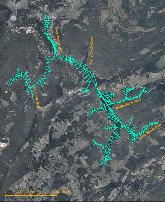
Figure 1. U. S. Geological Survey bathymetric data-collection lines, Deep Creek Lake, Garrett County, Maryland, 2007.

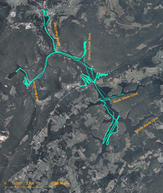
Figure 2. Maryland Department of Environment bathymetric data-collection lines, Deep Creek Lake, Garrett County, Maryland, 2008.

Methods

Bathymetric data were collected using a 24-ft (foot), aluminum-hull work boat. Surface-water temperature during data acquisition was a constant 72° F (degrees Fahrenheit) (22° C/degrees Celsius). Temperature profiles collected on September 18th, 2000 show temperature variations throughout the lake at various depths between 50 and 67.6° F (10 and 19.8° C) (Matthew C. Rowe, Maryland Department of the Environment, written commun. June 7, 2007). Such temperature variations would affect the velocity of sound in water (and thus measured depth) by approximately plus or minus 0.44 percent.

The data were collected using a Lowrance LMS480 fathometer and global positioning system (GPS) enhanced with a wide-area augmentation system (WAAS). This was referenced to the world geodetic system of 1984 (WGS-84) and was capable of producing latitude, longitude, and single beam echo-sounded depth data at a rate of one data point per second. The transducer operated at 200 kilohertz with a 20-degree cone angle.

Data-collection path lines were designed to maximize lake-surface coverage, and a zigzag pattern was used in most locations. In areas where lake width permitted supplemental data collection, path lines were run near shore and near the center-of-channel. The average boat speed was approximately 2.0 knots or 2.3 miles per hour. Data collection occurred once every second. At this speed and data-acquisition rate, a data point was generated every 3.4 ft of linear distance traveled on each transect, thus producing a dataset of nearly 140,000 data points across the study area.

Data Processing

Bathymetric data collected in September and October 2007 were normalized to account for the depth of the transponder below the water surface (0.8 ft). Because personnel, work stations, and equipment placement in the boat remained constant throughout the study, the transducer depth also remained relatively constant. The data also were normalized to the full-pool level of the lake (2,462 ft referenced to the National Geodetic Vertical Datum or NGVD of 1929) to account for changes in lake-surface elevation during the survey. From September 27 to the end of data collection, the lake level was measured with an electric tape from a reference point on the bridge across Meadow Mountain Run. The level was measured in the morning before launching and in the evening after completion of the day’s data collection. The elevation of the reference point was later determined by standard leveling techniques. The data collected by MDE in July and August of 2008 were appended to the bathymetric data collected by the USGS in September and October of 2008 to create a dataset of nearly 146,000 points.

Once the USGS and MDE data were combined, depth data were converted to land-surface elevations by subtracting depth from the full-pool elevation. The dataset was supplemented by land-surface elevations within an extended buffer surrounding the lake. These elevations were derived from the National Elevation Dataset (Gesch, 2007; Gesch and others, 2002). A lake-bottom surface was created through the interpolation of elevations between measured points along the lake bottom. This process, performed using the TOPOGRID command in ArcGIS, uses a locally adaptive approach to an iterative finite-difference interpolation gridding technique (Hutchinson, 1988). The process calculates values for grid cells at increasingly finer resolutions, starting with a coarse initial grid and successively halving the grid spacing until the final user-specified resolution is reached (Golub and van Loan, 1983). Cell values are generated by linear interpolation from the preceding grid. At each resolution, the elevation value at a given cell represents an estimate of the average of the actual surface elevation across that particular grid cell. Eventually, the resolution is sufficiently fine for there to be little or no data-point averaging. At this point, the grid is considered to be stable and all information has been extracted from the source data (Hutchinson, 1996). The resulting surface model of the lake bottom is a smoothed representation of exact point measurements made during the survey. The spot-depth map and lake bottom elevation grid are generalizations used to aid in visualization of the dataset (fig. 3 ). The survey points establish a measured base and allow for flexibility and consistency in determining future interpolation methods and comparisons.

The bathymetric survey points, their latitude and longitude in decimal degrees, lake depth in feet, and the lake-surface elevation in feet are shown in table 1.
(Table 1: Text version)

References Cited

Gesch, D.B., 2007, Chapter 4--The National Elevation Dataset, in Maune, D., ed., Digital Elevation Model technologies and applications: The DEM Users Manual, 2d ed.: Bethesda, Maryland, American Society for Photogrammetry and Remote Sensing, p. 99-118, accessed November 9, 2009 at http://topotools.cr.usgs.gov/pdfs/Gesch_Chp_4_Nat_Elev_Data_2007.pdf.

Gesch, D.B., Oimoen, M., Greenlee, S., Nelson, C., Steuck, M., and Tyler, D., 2002, The National Elevation Dataset: Photogrammetric Engineering and Remote Sensing, v. 68, no. 1, p. 5-11.

Golub, G.H., and Van Loan, C.F., 1983, Matrix Computations: Baltimore, Maryland, Johns Hopkins University Press, 476 p.

Hutchinson, M.F., 1998, Calculation of hydrologically sound digital elevation models, Third International Symposium on Spatial Data Handling, August 17-19, Sydney: Columbus, Ohio, International Geographical Union, p. 117-133.

Hutchinson, M.F., 1996, A locally adaptive approach to the interpolation of digital elevation models in Proceedings of the Third International Conference/Workshop on Integrating GIS and Environmental Modeling, Santa Fe, New Mexico, January 21-26, 1996: Santa Barbara, California, National Center for Geographic Information and Analysis, 6 p.

Bathymetry Map

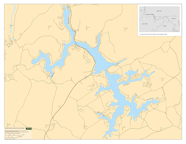
Figure 3. Bathymetric map of Deep Creek Lake, Garrett County, Maryland, 2007-08
Click to download full-sized map.

Note: To print the full-sized version, open the PDF in a PDF reader and print to a large-format printer.