
|
List of Figures - Click on figure for larger image.
 |
Figure 1. Location map showing the continuous resistivity profiling (CRP) survey tracklines. The different colors indicate different days of surveying. The background image is from ArcGIS Online, ESRI_Imagery_World_2D, accessed September 2010. Copyright 2009, ESRI, i-cubed, GeoEye. |
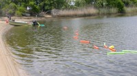 |
Figure 2. Continuous resistivity profiling (CRP) streamer deployed behind the survey boat. Foam flotation is attached to the cable between each electrode. Photo by John Bratton, NOAA. |
 |
Figure 3. Continuous resistivity profiling (CRP) data acquisition system in the survey boat. The yellow box to the left is the AGI SuperSting R8 Resistivity Meter, the black box in the middle manages the battery power to the system, and the yellow box to the right contains the Lowrance GPS-enabled fathometer. Photo by John Bratton, NOAA. |
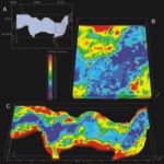 |
Figure 4. Perspective views of a horizontal slice at 10 meters below zero elevation through a three-dimensional (3D) solid model created from the continuous resistivity profile (CRP) data in Dynamic Graphics' EarthVision software. Part A is a plan view map where the gray lines represent the CRP tracklines, the blue polygon represents the extent of the 3D model shown in part C, and the red box indicates the extent of the 3D model shown in part B. The color bar applies to both parts B and C, with resistivity values in ohm-meters. In each map, along the northern part, small black symbols outlined in white represent offshore piezometer sampling locations. The white dashed lines in part B approximate paleochannel margins. |
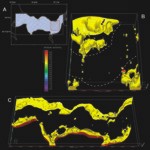 |
Figure 5. Perspective views of three-dimensional (3D) surface of equal resistivity (7 ohm-meters) derived from a solid model created from the continuous resistivity profile (CRP) data in Dynamic Graphics' EarthVision software. Part A is a plan view map where the gray lines represent the CRP tracklines, the blue polygon represents the extent of the 3D model shown in part C, and the red box indicates the extent of the 3D model shown in part B. The color bar applies to both parts B and C, with resistivity values in ohm-meters. In each map, along the northern part, small black symbols outlined in white represent offshore piezometer sampling locations. The white dashed lines in part B approximate paleochannel margins. |
|


