Click on figure for larger image.

Figure 2. Location map showing the continuous resistivity profiling tracklines of the surveys in May and September 2008 in Great South Bay, Long Island, New York.

Figure 3. Photograph of the National Park Service boat used for data collection in Great South Bay. Photograph by VeeAnn Cross, U.S. Geological Survey.

Figure 4. Photograph of the continuous resistivity profiling streamer deployed behind the R/V Terrapin (photograph is from a different survey). Foam flotation is attached to the cable between each electrode. Photograph by John Bratton, National Oceanic and Atmospheric Administration.

Figure 5. Photograph of the continuous resistivity profiling data acquisition system in the U.S. Geological Survey R/V Terrapin (photograph is from a different survey). The yellow box on the left of the photograph is the AGI SuperSting R8 resistivity meter, the black box in the middle manages the battery power to the system, and the yellow box on the right side contains the Lowrance GPS-enabled fathometer. Photograph by John Bratton, National Oceanic and Atmospheric Administration.

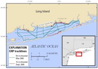
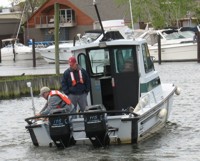
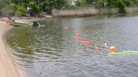
Data collection and processing methods are described here for continuous resistivity profiling (CRP) data collected in Great South Bay (fig. 2). These data were collected during two separate cruises in 2008. From May 19 to May 22 data were collected using a 50-m streamer towed from a National Park Service (NPS) boat (fig. 3). From September 22 to September 25 data were collected using a 15-m streamer towed by the USGS R/V Terrapin (fig. 4).

The CRP data were collected using methods similar to those described by Cross and others (2008, 2010 and 2011). In this study, over 200 kilometers (km) of CRP data were collected to image the fresh-saline groundwater interface in sediments beneath Great South Bay. Table 1 summarizes the data collection.

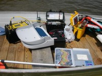
Data were collected using an Advanced Geosciences, Inc. (AGI) SuperSting R8 Marine resistivity system (figs. 4 and 5) configured with two different resistivity streamers during two separate survey periods. The AGI 50-meter streamer is an 11-electrode array with electrodes spaced 5 m apart. The two source electrodes are graphite, while the nine receiver electrodes are stainless steel. This streamer was used in May 2008. The AGI 15-m streamer is an 11-electrode array with electrodes spaced 1.5 m apart. As with the 50-m streamer, the two source electrodes are graphite, while the nine receiver electrodes are stainless steel. This streamer was used in September 2008. The longer streamer was used to collect regional data in deeper water along shore-parallel and long cross-bay transects with lower resoution but greater depth penetration. The shorter streamer was used to collect representative local data in select onshore–offshore transects with higher resolution but shallower depth penetration. In both cases, foam flotation was attached to the cable between each electrode to keep the cable at or near the surface, while allowing the electrodes to hang a little below the water surface and helping to keep the electrodes in the water in mildly choppy seas. The depth of penetration of these systems is approximately 25 percent of the towed cable length. A dipole-dipole configuration was used for the data collection in which two fixed-current electrodes were assigned, and voltage potentials were then measured between electrode pairs in the remaining nine electrodes.

The initial values recorded by the system are measured apparent resistivity values. A two-dimensional (2D) resistivity model takes into account resistivity changes in the vertical and horizontal directions along a survey line, while assuming resistivity remains constant perpendicular to the survey line (Loke, 2000). The apparent resistivity data undergo an iterative inversion process, which produces a resistivity profile that is most consistent with the measured values. EarthImager 2D inversion software is used to divide the subsurface into a number of rectangular blocks. The resistivity of each of these blocks is determined, creating an apparent resistivity pseudosection that is consistent with the measured apparent resistivity values. By constraining the model with the water-depth profile, where water thickness (depth) and resistivity are known from field measurements, a more accurate subsurface-resistivity profile can be generated. Processing parameters such as the type of inversion process, number of iterations, and amount of roll-along data overlap, can be used to further constrain the modeling. The data, both raw and processed, including metadata compliant with Federal Geographic Data Committee (FGDC) standards, can be accessed through the Data Catalog page. The metadata files give full details on the parameters used to process the data.

The shipboard control and logging system used for the data collection of the resistivity streamer was an AGI SuperSting R8 Marine resistivity meter (fig. 5). Current was injected into the water/sediment system approximately every 3 seconds through the source electrode pair at the front end of the streamer, and eight apparent resistivity values representing eight depth levels were recorded for each current injection. A Lowrance LMS-480M Global Positioning System (GPS) with an LGD-2000 GPS antenna and a 200-kilohertz fathometer transducer with a temperature sensor were also attached to the system in order to acquire navigation and measure water depth.

At the end of each day of data acquisition, the CRP and navigation/depth data were downloaded from the SuperSting system to a laptop computer running AGI's Marine Log Manager software. The data were then transferred to a processing computer to check the quality of the navigation data and process the CRP data using the AGI Marine Log Manager and EarthImager 2D software packages. The Marine Log Manager software was used to merge the navigation file (file extension GPS) with the raw resistivity data (file extension STG), resulting in a linearized resistivity data file (file extension STG) and a file containing the depth and temperature data when available (file extension DEP). These files are used as input to AGI's EarthImager 2D software for data processing.

The DEP files can be modified to include the water resistivity value measured at the time of surveying. Water samples were taken so that water salinity could be measured during each survey. For the May cruise, salinity was measured at 25.1. The average water temperature based on the Lowrance temperature sensor was 14 degrees Celsius. Using these values, a water resistivity value of 0.32 ohm-meters (ohm-m) was calculated for the May cruise. For the September cruise, salinity was measured at 25. The average water temperature in the bay based on the Lowrance temperature sensor was 19.45 degrees Celsius. Using these values, a water resistivity value of 0.29 ohm-m was calculated for the September cruise. These values were added to the appropriate DEP files used in processing all of the data.

EarthImager 2D version 2.2.8 was used to process the data files (STG and DEP) using the supplied CRP saltwater processing parameters, which have minimum and maximum allowable resistance and voltages appropriate for the marine environment. The EarthImager 2D CRP module is specifically designed to process large amounts of continuous resistivity data, as are typically acquired during marine surveys. The strategy the software uses for data processing could be described as a "divide-and-conquer" method, in which the long section of a single collection file is divided into many subsections. These subsections are individually inverted, and the processing culminates by assembling the individual sections into a single profile (Advanced Geosciences Inc., 2005). The output files from all of these steps are saved into an individual folder. For the purposes of this report, the linearized STG and DEP files used as input for the processing were saved, as well as three file types generated during processing. These include:

• JPEG images of the complete resistivity profile. Both long (uncompressed, same horizontal scale) and short (compressed to fit on a single page therefore having different horizontal scales) versions are available for each line.
• Text files of the processed resistivity data. These include XYZ files in which X = distance along line, Y = depth, and Z = resistivity value and LLT files, which contain longitude, latitude, depth, and resistivity values.
• A file with the INI extension containing the processing parameters used. This INI file can be loaded prior to subsequent file processing to ensure that the same parameters are used for all files or to verify the processing parameters used.

The JPEG images resulting from the EarthImager 2D processing were saved with the default color scale. This color scale ranges from blues to reds with reds representing the higher resistivity values corresponding to fresher (less saline) groundwater. The color scale within each image is maximized for the range of resistivity values from that survey line.

In addition, to more easily compare different resistivity profiles, the MathWorks, Inc. MATLAB software was used to combine the XYZ and DEP files to generate JPEG images with a common color scale for all survey line files. Within these images, the polarity of the color scheme is the same as that of the EarthImager 2D JPEGs, in that the colors range from blue to red with reds indicating higher resistivity values. MATLAB was also used to plot the data in an attempt to display the JPEG images with a common vertical and horizontal distance scale. Rounding errors in figure-size scaling prevents exact reproducibility of scale in the horizontal direction for the images.

Both the EarthImager 2D and the MATLAB JPEG images can be accessed from the Profile Previews pages.

MATLAB was also used to remove the water-column resistivity data from the XYZ files based on the water depth data in the DEP data files. Both the DEP and XYZ data were interpolated within MATLAB to extract a resistivity value for the sediment/water interface. The interpolated value, along with the measured values within the sediment, was exported to the modified XYZ data file. All the CRP lines were processed, and the results were combined into two shapefiles based on survey acquisition streamer and time period (allgsb_resbsed_may08 and allgsb_resbsed_sept08) and are available from the Data Catalog page.

Finally, a Visual Basic 6 program was created and used to combine the linearized STG file with the DEP file from each survey line to create a data file in RES2DINV format for users of that software package. These files are available from the Data Catalog page.