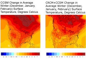
Data

Geographic Information System (GIS) Data

Our analysis involved the use of data from numerous GIS sources, as listed in table 2. We used several GIS layers to create hydrologic response units (HRUs), or areas where the hydrologic response is assumed to be the same, for use in the Precipitation Runoff Modeling System (PRMS). We also used GIS to estimate parameter values for each HRU as explained in the "Methods" section.

Flow Data

To calibrate and test a PRMS model, a daily flow record is required. A flow record of 20–30 years is ideal for model calibration and validation, and the minimum data requirement is about 6–7 years. Flow records were not available for the mouths of any of the four watersheds of interest. Therefore, for each watershed, we identified a suitable gaged calibration sub-watershed or similar neighboring watershed, and used its flow record to develop the model. This process will be described in more detail in "Methods." The four streamflow-gaging stations used are listed in table 3.

Historical Climate Data

Other required data for hydrologic modeling included historical minimum temperature (TMIN), maximum temperature (TMAX), and total precipitation (PRECIP) at a daily time step. For these inputs, we used the synthetic weather grid data prepared by the Climate Impacts Group (CIG), University of Washington, as a part of the Columbia Basin Climate Change Scenarios Project (CBCCSP) (Hamlet and others, 2010). The gridded data, hereafter referred to as CIG data, are based on the Parameter-elevation Regressions on Independent Slopes Model (PRISM), which is an interpolation of historical station data with consideration of orographic effects, temperature inversions, and coastal effects (Daly and others, 2002; Salathe and others, 2007; PRISM Climate Group, 2012). CIG data points inside of or within 5 km of each calibration sub-watershed were averaged into a single data file.

This approach has several advantages. Most importantly, climate inputs are representative of the entire sub-watershed, avoiding errors associated with generalization from a few weather stations to a large area. Orographic effects, which are considered in the CIG data, are especially important in mountainous and complex terrain such as that of the Coast Range. CIG data also have no gaps, so patching was not required, and the CIG period of record is long (1915–2006). Finally, using CIG historical climate data to calibrate all four coastal watershed models improved model comparability, because the smallest watersheds had no good candidates for historical weather stations, and had to be calibrated with CIG data. To confirm that the CIG data accurately reflected the historical record in our study areas, we selected nine weather COOP (COoperative Observer Program) stations that were inside of or within 10 km of the four calibration sub-watersheds (COOP ID 350471, 354133, 356820, 358182, 358494, 358833, 453333, 455774, and 456914). We then compared PRECIP, TMAX, and TMIN values from each station to the values from its closest CIG grid point. Across the nine stations, the mean coefficients of determination (R²) from simple linear regressions for PRECIP, TAMX, and TMIN were 0.92, 0.97, and 0.99, respectively. This high level of fit supported the decision to use the CIG data.

Future Climate Scenarios

The other key datasets in this analysis were the future climate scenario outputs. We selected scenarios from the North American Regional Climate Change Assessment Program (NARCCAP) to increase compatibility with other aspects of the larger project on estuaries and climate change, and because they are state-of the-art scenarios. These climate change simulations are produced by embedding Regional Climate Models (RCMs) within global-scale Atmosphere-Ocean General Circulation Models (AOGCMs) (North American Regional Climate Change Assessment Program, 2011a). By combining the models, the resolution of the outputs is improved greatly over those of an AOGCM alone. Outputs from an AOGCM and an AOGCM-RCM pair are shown in figure 4. The enhanced resolution is especially apparent over the Rocky Mountains.

Figure 4. Examples of North American Regional Climate Change Assessment Program scenario outputs. Outputs from an Atmosphere-Ocean General Circulation Model (AOGCM) are shown on the left, and outputs from an AOGCM-Regional Climate Model (RCM) pair are shown on the right (North American Regional Climate Change Assessment Program, 2011b).

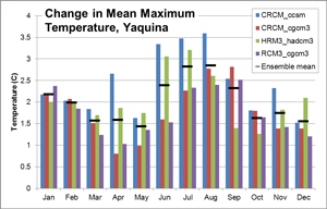
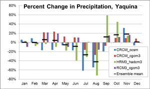
Because of limited resources, the NARCCAP focuses on developing as many AOGCM-RCM pairs as possible, rather than using multiple carbon emissions scenarios. The NARCCAP selected a single emission scenario, A2, which is at the higher end of the emissions scenarios, though it is not the highest. Like the other carbon emission scenarios commissioned by the Intergovernmental Panel on Climate Change, it is described in Nakicenvoic and others (2000). NARCCAP researchers argue that selecting a single high-emission scenario is reasonable because if we plan for extreme circumstances, we will also be prepared for moderate changes. The recent trajectory of carbon emissions (1990 to 2011) also best fits a fairly high emission scenario (North American Regional Climate Change Assessment Program, 2011c). Although the NARCCAP eventually will release many different AOGCM-RCM simulations, at the time of this research (2012) only four were completed for our reference period (1971–1995) and a future period (2041–2065). These simulations are listed in table 4. We did not force the models with the ensemble mean, because this masks the variability of each scenario, and we were interested in seeing a range of possible future outcomes. Daily data for each watershed were extracted from the North American Regional Climate Change Assessment Program web site by Darrin Sharp at the Oregon Climate Change Research Institute (OCCRI), Oregon State University. All the data points within a bounding box for each watershed were averaged to produce mean values for that watershed. Parameters used were TASMAX/TASMIN (maximum and minimum daily surface air temperature) and PRECIP (precipitation). The precipitation value was reported every 3 hours, and had to be aggregated and averaged to compute a daily value.

Figures 5 and 6 show the changes in maximum daily temperature and total daily precipitation from the reference period to the future period in an example watershed (Yaquina Bay watershed). All four scenarios show increasing mean temperatures from the reference period to the future period (fig. 5), with CRCM-CGCM3 and HRM3-HADCM3 showing larger increases in summer. However, there is much less consistency in modeled changes in precipitation (fig.6). In most months, some models show decreases in precipitation, and some show increases. Only in August and November is there agreement as to the direction of change. Changes in input data from the reference period to the future period vary among the watersheds, but this pattern of greater consistency in temperature than precipitation is present in all four study areas. Because the relation between precipitation and flow is direct in these low-permeability, rain-dominated watersheds, such discrepancies in predicated precipitation make it difficult to model future runoff confidently.

Figure 5. Absolute change in mean maximum daily temperatures from reference period (1971–1995) to future period (2041–2065) by month, in the Yaquina Bay watershed, Oregon.

Figure 6. Percent change in mean total daily precipitation from reference period (1971–1995) to future period (2041–2065) by month, Yaquina Bay watershed, Oregon.

First posted February 28, 2013