Results

Model Performance

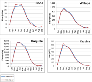
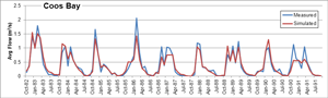
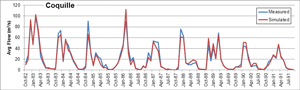
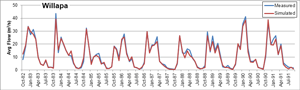
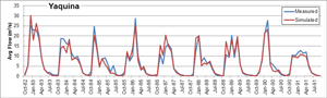
Four modeled goodness-of fit metrics: NSE, correlation coefficient, index of agreement, and annual percent bias are shown in table 10. All scores are based on daily data. Mean simulated and measured monthly flow rates are shown in figure 16, and a monthly hydrograph for each sub-watershed for October 1982–September 1991 is shown in figures 17 through 20.

Together, the figures and table show that the calibration sub-watersheds performed well. For example, annual percent bias was less than plus-or-minus 5 percent in all cases, and the NSE was 0.8 or greater for all watersheds except for the Coos Bay South Slough calibration sub-watershed. The Coos Bay South Slough calibration sub-watershed performed more poorly than the other watersheds by all measures, which is not surprising, given its short period of record, geologic composition, small area, and the likely influence of tides close to the ocean. Peak flows were underestimated in this sub-watershed (fig. 17),in the Willapa Bay sub-watershed (fig. 19), and, to a lesser extent, in the Yaquina Bay sub-watershed (fig. 20). This systematic underestimation bias in peak flows could be due to an underlying weakness in the PRMS model, precipitation under-catch, or some combination thereof. Overall, however, performance was satisfactory, because the NSE scores were above the 0.6 cutoff suggested in Choi and Beven (2007).

Figure 16. Mean monthly performance of calibrated models.

Figure 17. Monthly hydrograph of Coos Bay calibration sub-watershed, Oregon, October 1982–September 1991.

Figure 18. Monthly hydrograph of Coquille River calibration sub-watershed, Oregon, October 1982–September 1991.

Figure 19. Monthly hydrograph of Willapa Bay calibration sub-watershed, Washington, October 1982–September 1991.

Figure 20. Monthly hydrograph of Yaquina Bay calibration sub-watershed, Oregon, October 1982–September 1991.

PRMS Outputs with Climate Scenarios

Percent Change in Monthly Mean Flow Rate from Reference Period to Future Period

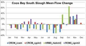
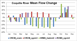
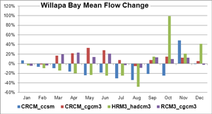
The outputs produced by forcing the ungaged study watershed models with NARCCAP scenarios are summarized in figures 21 through 30. Figures 21 through 24 show the percent change in mean monthly flow from the reference period to the future period. Each watershed has its own chart, and the different NARCCAP scenarios are symbolized by contrasting colors. The inconsistency in the direction of change among the scenarios is striking. In most months, CRCM-CGCM3 and RCM3-CGCM3 (which share an AOGCM; see table 4) show increasing trends, whereas the other two scenarios show decreasing trends throughout much of the year. Only in October and November is there more agreement among the models; in these months, almost all models show increasing mean flow. This is clear in figure 25, which shows the inter-watershed mean percent change for each month. However, the September values for the Coquille River watershed do not agree with the general pattern (fig. 22). This may be because the Coquille River watershed is the southernmost in this study, and is likely to have differing future precipitation and temperature. In figure 26, the ensemble mean of the four climate scenarios is displayed, and the different colored bars represent watersheds rather than scenarios. Here, the mean increases in October and November flow are even more apparent. Decreases in summer flow (July and August especially) also become evident in figure 26, because although the direction of the trend varies among the scenarios for most watersheds in this period, the magnitude of the decreasing trends is much greater, and so the ensemble mean shows a decrease.

Figure 21. Percent change in mean monthly percent flow from reference period (1971–1995) to future period (2041–2065), Coos Bay South Slough watershed, Oregon.

Figure 22. Percent change in mean monthly percent flow from reference period (1971–1995) to future period (2041–2065), Coquille River watershed, Oregon.

Figure 23. Percent change in mean monthly percent flow from reference period (1971–1995) to future period (2041–2065), Willapa Bay watershed, Washington.

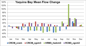Figure 24. Percent change in mean monthly percent flow from reference period (1971–1995) to future period (2041–2065), Yaquina Bay watershed, Oregon.

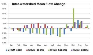Figure 25. Percent change in mean monthly percent flow from reference period (1971–1995) to future period (2041–2065), averaged across all four study-area watersheds.

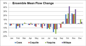Figure 26. Climate scenario ensemble mean change in mean monthly percent flow from reference point (1971–1995) to future period (2041–2065), by study-area watershed.

Changes in Monthly Coefficient of Variation (CV) from Reference to Future Period

As shown in figures 27 and 28, CV shows a small increase in most months (September–May) and for most scenarios. In July and August, however, CV decreases, probably because of fewer precipitation events and, thus, lower and steadier flow rates. The most dramatic change, however, is a spike in September CV in the HRM3-HADCM3 and RCM3-CGCM3 scenarios (fig. 27). Even when all scenarios are averaged (fig. 28), this increase is the most notable result. The increase could be owing to the fact that more rainstorms and associated variability in flow will be more likely in September with climate change.

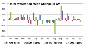Figure 27. Graph showing percent change in monthly coefficient of variation (CV) from reference period (1971–1995) to future period (2041–2065), averaged across all four study-area watersheds.

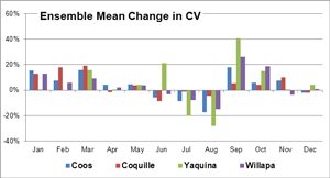Figure 28. Graph showing climate scenario ensemble mean change in monthly coefficient of variation (CV) from reference period (1971–1995) to future period (2041–2065), by study-area watershed.

Changes in Other Indices from Reference Period to Future Period

We also investigated percent change in the top 5 percent of flow (fig. 29) and in the 7-day low flow (fig. 30). The Willapa Bay and Yaquina Bay watersheds show likely increases in top 5 percent of flow because all four models agree as to sign, and three of four scenarios show increases of more than 5 percent from the reference period to the future period. The percent change in 7-day low flow shows less agreement among climate scenarios, although there is an ensemble mean decrease for all watersheds except the Yaquina Bay watershed. The differing value in the Yaquina Bay watershed may arise from local variability in the RCMs. In an investigation of GCM downscaling techniques for hydrologic modeling, Wood and others (2004) determined that data downscaled with an RCM gave hydrologically probable results only after bias correction. Poor resolution of realism of the RCMs also may be a factor here. Given the higher degree of uncertainty associated with these low flows, and the lack of a strong signal, it is better not to rely on the ensemble mean in this case.

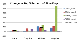Figure 29. Graph showing percent change in flow in top 5 percent of days from reference period (1971–1995) to future period (2041–2065).

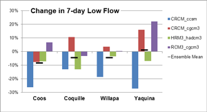Figure 30. Graph showing percent change in 7-day low flow from reference period (1971–1995) to future period (2041–2065).

Uncertainty Analysis Results

PRMS Parameter Uncertainty

Figures 31, 32, 33, and 34 show the uncertainty owing to model parameters in the four calibration sub-watersheds. In each figure, the red points represent observed flow values, and the gray region shows the range of values generated by the randomly generated parameter sets that met performance criteria described in ”Methods”. For each model, results are displayed on a linear scale (a in figures) and logarithmic scale (b in figures), so that high- and low-flow uncertainty can be readily seen. In each model, the same 6-year period (October 1984–September 1990) is shown, and the X- axis represents number of days. The logarithmic charts show that the uncertainty of low flow is high, which agrees well with previous research (for example, Chang and Jung, 2010). The smallest calibration sub-watershed, for the Coos Bay South Slough, shows consistent under-prediction of the high flow, regardless of the parameter set used. The range of possible values does not include the observed data point in several cases. This may suggest a systematic bias in PRMS that becomes more obvious in smaller watersheds, and it also may be related to a possible underestimation of precipitation data.

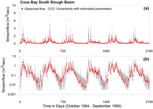Figure 31. Precipitation Runoff Modeling System parameter uncertainty for Coos Bay calibration sub-watershed, Oregon. (a) is a linear scale, and (b) is a logarithmic scale.

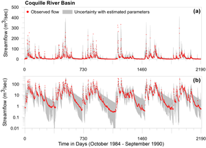Figure 32. Precipitation Runoff Modeling System parameter uncertainty for Coquille River calibration sub-watershed, Oregon. (a) is a linear scale, and (b) is a logarithmic scale.

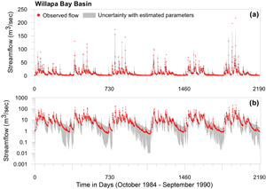Figure 33. Precipitation Runoff Modeling System parameter uncertainty for Willapa Bay calibration sub-watershed, Washington. (a) is a linear scale, and (b) is a logarithmic scale.

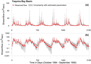Figure 34. Precipitation Runoff Modeling System parameter uncertainty for Yaquina Bay calibration sub-watershed, Oregon. (a) is a linear scale, and (b) is a logarithmic scale.

NARCCAP Uncertainty

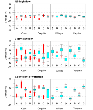
To assess uncertainty associated with climatic data, we used the random parameter sets that performed well in the calibration sub-watershed to create multiple models of the ungaged watersheds, which we then forced with the NARCCAP climate scenario data. Statistics from the resulting outputs are shown in figures 35 and 36. In figure 35, the percent change in each statistic (top 5 percent of flow, 7-day low flow, and CV), from the reference period to the future period, is shown for each watershed and each climate scenario. The lines in the middle of the boxes denote the median values and the upper and lower boundaries of the boxes show the 25^th and 75^th percentiles, respectively. The red diamond symbol indicates outliers. There are considerable differences among the scenarios for each statistic and each watershed. Percent change in CV for the Yaquina Bay watershed is an extreme example of such discrepancies; the ranges of values for each scenario do not overlap.

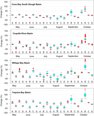
Figure 36 shows the percent change in flow for each month, by watershed, with a separate box plot for each scenario. As in figure 35, the lines in the middle of the boxes denote the median values, the upper and lower boundaries of the boxes show the 25^th and 75^th percentiles, and red diamonds represent outliers. In many cases, there is little overlap in the range of changes among the four scenarios; this is especially evident in March and April, when RCM3-CGCM and CRCM-CGCM3 show increases, and HRM3-HADCM3 and CRCM-CCSM show decreases. The HRM3-HADCM3 model, which shows the greatest increases in autumn flow, also has the greatest range of results.

These boxplots, with their lack of agreement among models, confirm that the selection of climate models, rather than hydrologic parameter values, is the greatest source of uncertainty. Many previous studies have reached the same conclusion (for example, Wilby and Harris, 2006; Graham and others, 2007; Maurer, 2007; Prudhomme and Davies, 2009; and Chang and Jung, 2010).

Figure 35. Box-and-whisker plots showing changes in top 5 percent high flow, 7-day low flow, and coefficient of variation for four study areas. The lines in the middle of boxes denote the median values, and the upper and lower boundaries of the boxes show the 25th and 75th percentiles, respectively. The red diamond symbol indicates outliers. A is for RCM3-CGCM, B is for HRM3-HADCM3, C is for CRCM-CGCM3, and D is for CRCM-CCSM.

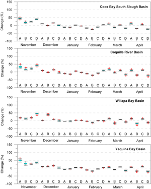Figure 36. Box-and-whisker plots showing changes in monthly runoff for four study areas. The lines in the middle of boxes denote the median values, and the upper and lower boundaries of the boxes show the 25th and 75th percentiles, respectively. The red diamond symbol indicates outliers. A is for RCM3-CGCM, B is for HRM3-HADCM3, C is for CRCM-CGCM3, and D is for CRCM-CCSM.

First posted February 28, 2013