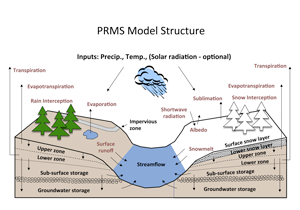
Methods

Precipitation Runoff Modeling System (PRMS)

We selected the Precipitation Runoff Modeling System (PRMS) because it has been used in many investigations and regularly improved (Markstrom and others, 2008). PRMS also has been used successfully in climate change impact assessments around the world (for example, Burlando and Rosso, 2002; Legesse and others, 2003; Bae and others, 2007; Qi and others, 2009; Chang and Jung, 2010; Jung and Chang, 2011).

PRMS is a semi-distributed, physically based surface runoff model developed by the USGS (Leavesley and others, 1983; Leavesley and Stannard, 1995). The model is composed of Hydrologic Response Units (HRUs) that are assumed to have a homogeneous hydrological response. PRMS computes a daily water balance for each HRU, and the sums of water and energy balances, weighted by each HRU’s relative area, yield daily watershed output values for flow, soil moisture, evapotranspiration, and other variables (Hay and others, 2009). The processes and water storage zones represented by equations in PRMS are shown in figure 7.

Figure 7. Processes modeled by Precipitation Runoff Modeling System.

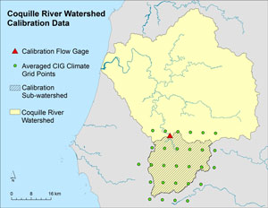
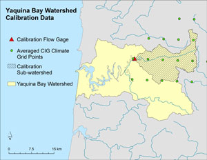
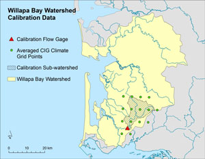
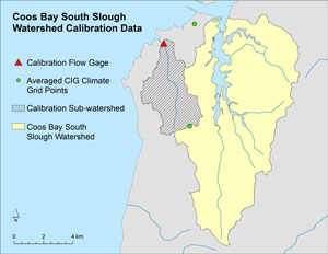
Calibration Flow Gage Selection

Because only a part of each estuary’s watershed was gaged, we used calibration sub-watersheds or neighboring similar watersheds in which the model outputs could be fitted to observed data. The calibrated parameter values then could be transferred to the ungaged watershed of interest. Several previous studies demonstrated the robustness of this approach (for example, Merz and Bloschl, 2004; Kay and others, 2006; Chang and Jung, 2010). When selecting calibration gages, we looked first for gaged sub-watersheds with the largest possible spatial and temporal coverage, and then for nearby watersheds with similar characteristics. We also avoided gages that were downstream of dams or major withdrawals. Calibration sub-watersheds for the Coquille River, Willapa Bay, and Yaquina Bay watersheds are shown in figures 8, 9, and 10. The Coos Bay South Slough watershed had no gaged sub-watershed, so we looked for a neighboring gaged watershed that was comparable in land use, elevation, area and other factors, and that had adequate temporal coverage. Selected calibration watersheds are shown in figure 11.

In the remainder of this report, these calibration regions are referred to as "sub-watersheds" to avoid confusion with the estuary watersheds of interest (though note that the Coos Bay South Slough calibration watershed is not a true sub-watershed). The best available flow station for Coos Bay South Slough had a shorter-than-ideal period of record for PRMS (table 3). Additionally, given its location, Coos Bay South Slough may be influenced by marine tides. These two factors, along with the small size of the sub-watershed, make it more difficult to simulate its flow accurately. After identifying the flow gages, we delineated sub-watersheds for each gage and for the entire watershed of interest using a 30-m USGS DEM.

Figure 8. Calibration data for Coquille River watershed, Oregon.

Figure 9. Calibration data for Yaquina Bay watershed, Oregon.

Figure 10. Calibration data for Willapa Bay watershed, Washington.

Figure 11. Calibration data for Coos Bay South Slough watershed, Oregon.

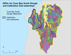
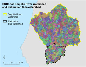
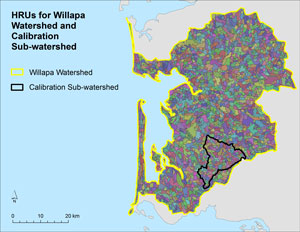
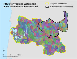
HRU Delineation

With our watershed boundaries identified, the next step was to delineate HRUs. To do so, we made minor modifications to a method described by Leanen and Risley (1997). For their PRMS model of the Willamette River Basin in Oregon, they delineated HRUs based on geology, hydrologic soil group, land use-land cover, and slope and aspect. Slopes were classified as 0–5 percent, 5–30 percent, and greater than 30 percent. When slopes were greater than 30 percent, they were further subdivided by aspect (north, south, east, or west).

Simplification steps were added to the Leanen and Risley (1997) method because the GIS layers currently available have much higher resolution than those available when the method was developed. Without simplification, tens of thousands of HRUs would be created for each watershed. To a point, increasing the number of HRUs improves accuracy, but above a threshold, model computation (or run) time increases, making it inefficient. We smoothed all input rasters, including slope, aspect, and LULC, with a majority filter. This filter replaces raster cell values based on the majority value of neighboring cells, which results in rasters with larger areas of homogeneity. When rasters are smoothed before they are used to define HRUs, fewer HRUs are ultimately produced. We also merged all HRUs with an area of less than 0.5 km² into a neighboring HRU. Resulting HRUs are shown in figures 12-15; the number of HRUs in each watershed and calibration sub-watershed are given in table 5.

Figure 12. Hydrologic Response Units (HRUs) for Coos Bay South Slough watershed, Oregon.

Figure 13. Hydrologic Response Units (HRUs) for Coquille River watershed, Oregon.

Figure 14. Hydrologic Response Units (HRUs) for Willapa Bay watershed, Washington.

Figure 15. Hydrologic Response Units (HRUs) for Yaquina Bay watershed, Oregon.

HRU Parameterization

For many PRMS parameters, such as land cover type and winter rain interception, we derived HRU values using GIS. We followed a detailed procedure on HRU parameterization prepared by the USGS (Lamorey, 2009). This method involves using zonal statistics to derive mean values for each parameter from various layers, many of which were functions of the USGS 2001 LULC layer, Soil Survey Geographic (SSURGO) soil data, or a DEM. For example, summer rain interception is calculated for each HRU based on the vegetation density, which is generated from the LULC map. The 20 HRU parameters derived directly or indirectly from GIS layers are listed in table 6. For a full description of the equations and GIS techniques involved in their derivation, see Lamorey (2009). We used static values for the geospatial parameters in reference and future periods, although land cover has changed during the study period, and likely will vary in the future periods. We did not have an LULC layer from the start of the reference period, nor were future LULC scenarios available. It was beyond the scope of the study to prepare such LULC layers, so static parameter values were used.

Model calibration

To calibrate the models, we used an iterative approach, and focused on adjusting parameters known to be sensitive in rain-dominated watersheds (U.S. Geological Survey, 2011). After each change, we assessed goodness of fit scores for a calibration period (table 3), reserving data from a verification period for a final evaluation. First, we focused on fitting the overall monthly water balance. Next, we attempted to fit high-flow periods. Finally, we attempted to fit low-flow periods. The parameters used in calibration, and their final value for each sub-watershed, are listed in table 7. Any parameters not listed here or in table 6 were assigned default values or were borrowed from USGS PRMS example models. We used default values for all parameters relating to snow accumulation and melt processes because these parameters are not sensitive in the rain-dominated coastal region. For more information about our calibration methods, see Chang and Jung (2010).

For one calibration sub-watershed, we also made adjustments to the historical CIG precipitation data. Direct manipulation of data inputs is generally not reasonable in hydrological modeling, but in this case, we had evidence that precipitation had been underestimated. A similar approach was used in assessing the effects of climate change on the hydrology of the Columbia River basin (Elsner and others, 2010). Specifically, in the calibration watershed for Willapa Bay, the annual ratio of CIG input precipitation to runoff (the runoff ratio) was 90 percent (table 8). This value is unrealistically high for a watershed with almost no impervious surfaces (Jung and others, 2011).

John Risley of the USGS recommended that we check these findings by estimating annual water budgets for this watershed using PRISM (Parameter-elevation Regressions on Independent Slopes Model) data, mean annual runoff depth from USGS annual data reports, and evapotranspiration estimates from the National Oceanic and Atmospheric Administration evaporation atlas (Farnsworth and others, 1982). We did so, and determined that the runoff ratio was also too high in this estimated water budget. Because the CIG data are derived from PRISM data, this is not surprising; both datasets share the same probable underestimation. The origin of the error may be under-catch in the weather stations used to derive the PRISM dataset; Legates and Deliberty (1993) estimate precipitation under-catch due to wind at more than 18 mm per winter month in this region. Fog drip, or occult precipitation, also has been estimated at 30 percent of total precipitation in a Douglas-fir forest in the northern Oregon Cascades (Harr, 1982), and it likely is important in the Willapa calibration sub-watershed as well. Therefore, we were justified in manipulating the precipitation inputs. We did this by multiplying all daily precipitation totals by 1.1 for September–April, but because of greater flow underestimation in summer, we used 1.3 for May, June, and August, and 1.4 for July. Improved runoff ratios are shown in table 8. Final model performance and calibration scores are presented in the results section.

After adjusting the CIG data and calibrating the sub-watersheds, we created models of the ungaged study watersheds using the same parameter values as were used in their respective calibration sub-watersheds.

Use of Climate Scenarios

As described in "Data", we obtained four NARCCAP simulations with complete daily records for a reference period (1971–1995) and a future period (2041–2065) (table 4). We used these data to force the calibrated models of the watersheds of interest (not the calibration sub-watersheds), and then compared reference and future outputs within models to calculate potential climate-induced runoff changes. Although we adjusted the precipitation inputs used to calibrate for Willapa Bay, we did not make any changes to the NARCCAP precipitation data because these different climate models would not necessarily share the same biases. The final outputs are summarized in "Results".

Uncertainty Analysis

All physical modeling of future conditions involves uncertainty. In hydrologic modeling, the primary sources of uncertainty are future climate and emissions scenarios. Precipitation is especially uncertain, and becomes more uncertain under high carbon emissions scenarios. Hydrological model parameter values also contribute to uncertainty (Praskievicz and Chang, 2009). Because PRMS uses many parameters, there is a strong likelihood of equifinality (Beven and Freer, 2001; Kirchner, 2006; Beven and others, 2007), which means that many different combinations of parameter values would all give rise to a statistically acceptable outcome. That is, one set of parameter values can score as well as another, even if it poorly reflects the physical reality. This results in uncertainty in the accuracy of future projections. Future climate models also introduce uncertainty to the simulations, especially in their precipitation estimates (fig. 6). To estimate the degree of uncertainty owing to PRMS and climate models, we conducted an uncertainty analysis.

After Chang and Jung (2010), we used a modified version of a method first suggested by Wilby (2005) to estimate the amount of uncertainty associated with each source. We selected 13 sensitive calibration parameters (table 9) and generated random values within the acceptable range for each parameter. A total of 20,000 random sets of parameters were generated for each calibration sub-watershed using Latin hypercube sampling in Matrix Laboratory (MATLAB®)(MathWorks, Natick, Massachusetts). Wilby (2005) used Monte Carlo sampling to generate his parameter sets, but we used Latin hypercube sampling instead because it has been shown to be more effective and efficient than Monte Carlo sampling (Davey, 2008). Each parameter set then was used in PRMS to simulate runoff, and the performance of each set was evaluated.

We then selected parameter sets that performed well for each calibration sub-watershed. Our criteria were: a Nash Sutcliffe Efficiency (NSE) coefficient of 0.8 or more, an index of agreement of greater than or equal to 0.85, and an annual percent bias of no more than plus-or-minus 10 percent. All performance scores were calculated using daily data. The NSE is a commonly used measure of goodness of fit in hydrologic models; as a model improves, its NSE approaches 1 (Nash and Sutcliffe, 1970). We changed the criteria slightly for the Coos Bay calibration sub-watershed because none of its 20,000 randomly generated parameter sets had an NSE of 0.8 or more. We lowered the cutoff for this sub-watershed to an NSE of 0.7, but kept the other criteria the same. After identifying the best parameter sets for each calibration sub-watershed, we used them to find the uncertainty associated with PRMS parameters.

To estimate uncertainty owing to climate models, we translated the best selected parameter sets to the ungaged study watersheds, and then forced these models with the four climate scenarios (table 4). We used these outputs to find uncertainty in estimated changes in monthly flow, coefficient of variation (CV), top 5 percent of flow, and 7-day low flow from the reference period to the future period. The CV is the ratio of the standard deviation to the mean, and frequently is used as a metric of variability in flow. The top 5 percent, or Q5, is the mean discharge rate of the 5 percent of days with the highest flow for each year. Seven-day low flow is the lowest 7-day running mean flow for each year (Chang and Jung, 2010). This metric is similar to 7Q10, a standard hydrologic metric, but is averaged over 30 years instead of 10 years. All findings are presented in "Results". Because all four climate scenarios use one emission scenario (as discussed in "Data"), uncertainty in climate projections is greater than the results indicate.

First posted February 28, 2013