
| Lake Pontchartrain Basin: Bottom Sediments and Related Environmental Resources |
Database Structure and Development (cont.)
Analytical Methods and Quality Control |
|
 |
|
Problems in Compiling Heterogeneous Data
The data in this study have been acquired from historical sources as well as from ongoing field programs. It is not feasible to apply the standard quality-control protocols that check on the details of sampling and analytical methodology (see Baker and Kravitz, 1992) to heterogeneous data. To rescue data while minimizing problems associated with data comparability, special batch screening techniques were used to identify and call attention to data that have unresolved problems. Although such tests do not necessarily prove that the data are in error, they alert users to data that should be reevaluated or confirmed before use in environmental characterization.
It is emphasized here that data anomalies are a normal and virtually inescapable part of any analytical program – especially one that deals with constituents in trace quantities. In recent years, increasing attention to data quality has greatly improved the reliability of analyses, especially from major Federal agency programs and their contractors. However, as will be seen in this chapter, comparability checks are necessary even for data from well-established laboratories.
Goal and Caveats: Maximizing Effective Data Resources
Inaccuracies in one or more constituents in a data set do not necessarily apply to other constituents from that set. Data screening, thus, has as goals maximizing both the spatial extent and reliability of the total data set to users. Although reasonable care has been taken in reporting and quality-screening data, the approaches used can only detect larger, relatively persistent and environmentally significant data quality problems. The responsibility for setting standards of quality for specific uses of the data cited here rests with the user.
Data Screening -- Discriminant Functions
Much is now known about the chemical composition and behavior of natural and contaminated sediments in estuarine ecosystems (Windom and others, 1989; Horowitz, 1991; Schwarzenbach and others, 1993). Expected internal chemical relationships and comparisons among data from different sources for given geographic areas help evaluate the quality of data sets. We used a series of operations and screening steps to explore heterogeneous historical data. These techniques were developed for use in studies of sediments from the Boston Harbor - Massachusetts Bay area (Manheim and Hathaway, 1991). In the present approach, batches of data are screened for completeness, internal consistency, and reasonableness in terms of geochemical parameters widely applicable to sediments.
One problem is incorrect or uncertain sample and station locations. For example, some latitudes and longitudes listed for stations near New Orleans were found to plot on land, rather than offshore. Fortunately, supplementary site descriptions available in the original reference made better site identification possible in this case.
|
Data sorting and concentration range assessment Guidelines published by Long and others (1995) define ranges of chemical concentrations found in estuarine sediments based on their toxicity levels. The ranges serve as estimates of contaminant levels that would produce adverse biological effects. These ranges were used as one method of screening the data in this Lake Pontchartrain sediment quality study. Data were evaluated by sorting analytical parameters by concentration and classifying the values into the ERL and ERM ranges from table 8. Comments were coded in the appropriate qualifier field to highlight samples that should be re-examined to determine whether the high concentrations were actually due to influence of specific contaminants or, simply, inaccuracies produced during the study. |
Table 8. Alert Ranges  click for larger view |
Discriminant functions employed here display inter-element relationships in ways that help discern potential data quality problems. Examples include batch plots of data on log/log scales in figures 7, 8, 9, and 10. Aluminum, organic carbon, and grain size (for example, "fines") have been used as normalizing constituents to attempt to quantify the tendency for contaminants to be associated with finer fractions of sediments (Horowitz, 1991). However, none of these are suitable for sediment quality control in the current study because consistent data are not available for these constituents. Instead, zinc, which is included in virtually all data sets, has been shown to have special attributes suited for quality control (Manheim, Buchholtz ten Brink, and Mecray, 1998). It has been used as the main comparator element in discriminant plots for metals in this work. Phenanthrene and other widely reported components have been used for similar discriminant plotting for organic constituents.
Figure 11 shows the linear relationship between iron and zinc for two data sets, one performed by hot nitric acid extraction, and the other (lab 2) by total dissolution. Divergence of the latter to higher iron values is expected because much insoluble iron is present in clay minerals. Scattering is attributed to local inhomogeneities and sample variability.
A third laboratory's data had no iron (Fe) values. The higher zinc (Zn) values are plotted in Figure 10 at approximate Fe ranges inferred for the types of sediments in question. Most of the high values as well as other data points showing anomalous Zn/Fe ratios have as a common feature proximity to the New Orleans shoreline region where samples close to discharge canals were documented earlier to have enhanced contaminant concentrations (Overton and others, 1986). The preponderance of the information indicates that the anomalous Zn values represent contaminant input rather than data quality problems for this area.
All the data shown in Figure 7 were performed by USEPA leachate methods utilizing standard hot nitric acid extraction, followed by spectrochemical end detection methods (USEPA, 1983). The data points plot well below the regression line derived from a national set of analyses (NS&T, 1996). The NS&T data set was based on total breakdown of the aluminosilicate mineral structure. The plot of data sets in Figure 7 shows drastic influence of different analytical methods, since the greater part of aluminum in silicate minerals like clay and feldspars is not extracted by nitric acid.
Differences between alternative methods are smaller but clearly discernible for chromium (fig. 8). The differences are still smaller for heavy metals such as copper (fig. 9) and are not significantly different for samples in which contaminants are a significant component. The purpose of leachate analyses is, in fact, discrimination against naturally occurring metals in clay and iron oxide matrices, thereby enhancing the relative contaminant signal. There are advantages and disadvantages to both the leachate and total dissolution approaches.
Examination of arsenic/zinc relationships (fig. 10) reveals wide divergence when compared with the national NS&T data set. One set (lab 1) showed consistency within expected local scattering. Data from lab 4 displayed distributions that could not be reconciled with the analytical methodologies employed or with data from well-controlled, independent studies in the same areas. Arsenic (As) data from this source were therefore assigned "warning" designations in the Qualifier field (see table B2 in appendix B). Samples from lab 2 and lab 3 utilized leaching techniques which yield lower metal recovery for naturally occurring As concentrations in clay minerals than do total recovery (TR) methods. Although leachate and TR methods may be valid on their own terms, the two kinds of data should not be combined to form regional means without normalization. (For more information on leachate versus TR methods, see Inorganic Chemistry).
| Sorting by grid area and element ratio | 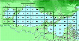 Figure 6. Guide to the AREA_CD_SQ field |
After anomalies were isolated by the methods indicated above, the data were checked against data from geographically controlled, independent sources. Mainly "standard data sets" with a high degree of available quality control were used for the comparisons. The purpose was to distinguish between anomalies that might be due to local contaminant sources and anomalous data of unresolved origin. An efficient method for comparing discriminant functions in constrained areas was sorting data according to geographical grid numbers (fig. 6). The data were first queried or sorted in descending order by the parameter in question to eliminate nondetects. Then, a consolidated table containing key station data including source information plus a limited number of analytical parameters (texture and heavy metals, for example) was sorted by grid number followed by the element in question and the discriminant ratio (for example, Zn/Cu). Discriminant ratios differing from those of well-qualified data by a factor of greater than 2.0 within grid squares were often a helpful indicator of significant anomalies. Where no problem resolution was available, data sets with a significant number of anomalous data were flagged with warning designations and excluded from interpretive output like histograms, statistical computations, or area plots.
The designation "W" in quality-control fields placed adjacent to data fields in the full database warns that the data in question appear to show unresolvable anomalies. "0" in a concentration field means that the constituent was analyzed and found to have a concentration below the detection limit for the method utilized. (Zeros are different, therefore, from blank fields, which show that the constituent was not measured). Other remarks in the quality-control fields provide comments relating to the data that may be helpful in interpreting or further evaluating the data. See appendix B for further explanations on quality control and codes.
Organic constituents were analyzed in the Louisiana Department of Environmental Quality resource studies of 1983-84 (Overton and others, 1984; Schurtz and St. Pé, 1984; Chew and Swilley, 1987). Except for samples close to the New Orleans shore, these were mostly below detection limits. The USEPA EMAP studies of 1991-94, used more recent methodologies with greater sensitivities (Macauley and Summers, 1998). These data yield more quantitative data on the many related congeners or organic species. (See Organic Components for further discussion).
| Forward to Sediment Texture & Bathymetry |
||
|
||