Scientific Investigations Report 2012–5062
Groundwater Flow ModelModel DescriptionGoverning Equations and Model CodeThe movement of groundwater through porous media is described by the following partial differential equation, which is based on Darcy’s law and the conservation of mass (McDonald and Harbaugh, 1988):
Note that specific storage (Ss) is the storativity (which is dimensionless) divided by the aquifer thickness (which has units of length), resulting in units of one over length (such as ft-1). Derivations of equation (1) can be found in Freeze and Cherry (1979) and Anderson and Woessner (1992). There is no evidence of large-scale horizontal anisotropy in the upper Klamath Basin; therefore, Kxx and Kyy are considered to be equal at any given location and Kxx and Kyy are replaced in this discussion by the single term Kh to describe horizontal hydraulic conductivity. Equation 1 represents the mass balance at a single point in space and time and generally cannot be solved analytically for practical applications involving transient conditions in complex three-dimensional systems. In practice, numerical methods are employed in which the partial differential equation 1 is approximated at a set of spatially discrete points in a process known as discretization. Equation 1 is then replaced by a set of simultaneous algebraic equations that describe the distribution of hydraulic head at each point, and flow through the system in response to this head distribution. These simultaneous equations are set up in matrix form and then solved. A variety of techniques are available to solve the set of simultaneous equations such as the preconditioned conjugate-gradient method of Hill (1990) and the algebraic multigrid solver of Mehl and Hill (2001). The upper Klamath Basin regional groundwater model was developed using MODFLOW-2000 (Harbaugh and others, 2000; Hill and others, 2000). MODFLOW-2000 is an extremely versatile groundwater-modeling code that has the capability to simulate transient groundwater flow in three dimensions subject to common boundary conditions used to represent hydrologic features such as streams, springs, drains, lakes, and evapotranspiration by phreatophytes. Discussions of the numerical technique used in this study, the finite-difference method, and MODFLOW-2000 can be found in McDonald and Harbaugh (1988), Anderson and Woessner (1992), Harbaugh and others (2000), and Hill and others (2000). DiscretizationAs mentioned above, numerical modeling requires that the model domain be divided into discrete regions or cells. For the model described in this report, the upper Klamath Basin was divided into cells with a lateral dimension of 2,500 ft by 2,500 ft aligned in a grid consisting of 285 east-west trending rows and 210 north-south trending columns (fig. 4). In the vertical dimension the model consists of three layers of varying thicknesses ranging from about 5 ft to 3,600 ft depending on topography and proximity to the edge of the model (fig. 5). The model layers are defined to correspond to hydrogeologic units where possible. The rectangular model grid comprises 179,550 cells of which 100,070 are active. Active cells are those for which groundwater flow is calculated and inactive cells are those that are outside of the modeled area. Hydrologic characteristics were defined for each cell in the model using the Layer-Property Flow (LPF) package of MODFLOW. Layers were formulated as confined (meaning transmissivity remains constant) to help linearize the model and improve numerical stability. Transient models require that time also be discretized into specific increments. MODFLOW requires two types of increments be defined, stress periods and time steps. A stress period is an interval over which specified boundary fluxes, such as recharge, and stresses (such as pumping) remain constant. Stress periods are subdivided into time steps. This further subdivision enables the model user to evaluate the timing of the hydrologic response to changes in stresses and also improves numerical stability. The upper Klamath Basin groundwater model has been set up to simulate quarterly stress periods from 1970 through 2004 water years. (Water years begin on October 1 and end on September 30. For example the 1970 water year starts October 1, 1969 and runs through September 30, 1970.) Each quarterly period is divided into five time steps. Parameterization of Subsurface Hydraulic CharacteristicsSimulating three-dimensional (3D) groundwater flow requires that the hydraulic properties of subsurface materials be represented in three dimensions. The hydraulic properties needed by the model are the hydraulic conductivity and the specific storage. The distribution of hydraulic properties in the upper Klamath Basin groundwater model is based on geologic mapping, stratigraphic information from water wells, and geophysical data. Sufficient information does not exist to accurately represent the full complexity of the spatial distribution of hydraulic properties. Therefore, the spatial distribution of hydraulic properties is simplified by defining zones in the model that generally follow hydrogeologic units, and in which hydraulic properties are considered uniform. The hydraulic conductivity and specific storage values assigned to each zone are initially based on independent information such as aquifer tests, specific-capacity tests, or literature values appropriate to the dominant rock type, and then refined during model calibration. The zonation of hydraulic properties used for the model is shown for each model layer in figure 6. The zones are primarily based on the dominant rock type in each region. Boundaries are based on the mapped geology and stratigraphic information from wells, as well as hydrologic information such as major changes in head gradients. The age of rock is also factored into the zonation. There is a general progression of the age of volcanic rocks at the surface across the upper Klamath Basin in which rocks generally increase in age from west to east. Quaternary volcanism is prominent along the western margin of the study area in the Cascade Range while the oldest (late Miocene) volcanic rocks most commonly are exposed in the northeast part of the basin (Sherrod and Pickthorn, 1992). Zonation was based on generalized geology described in Gannett and others (2007) but refined by more detailed 1:24,000-scale geologic mapping done by the Oregon Department of Geology and Mineral Industries and compiled by Jenks (2007). Quaternary Sediment (Qs)—This zone comprises the young surficial deposits in the uppermost parts of large sedimentary basins as well as alluvial deposits in stream valleys. These materials are usually shown as Quaternary sediment or alluvium on geologic maps. This zone occurs only in the uppermost layer of the model (layer 1). Layer 1 generally is about 45 ft thick in this zone. Quaternary Volcanic Deposits (Qv)—This zone encompasses areas mapped as Quaternary volcanic deposits in the Cascade Range south of the Klamath River as well as volcanic deposits associated with Medicine Lake Volcano at the southern end of the model. The materials primarily are basaltic and andesitic lava flows, but there are vent deposits and pyroclastic deposits as well. The thickness of these deposits is not well known and has been inferred from surface exposures and topography. It is limited to model layer 1. Qv ranges in thickness from 27 to 3,400 ft, being thickest in the Cascade Range. Quaternary Volcanic DepositsNorth (Qvn)—This zone corresponds to Quaternary volcanic deposits in the Cascade Range north of the Klamath River including the Crater Lake area. It is limited to model layer 1, and the lithology and thickness are similar to that of Qv. Quaternary Mazama Pumice (Qmp)—This zone consists of pumice and ash deposited during the climactic eruption of Mount Mazama, which formed Crater Lake. The unit is limited to model layer 1 in the northern part of the model just east of Crater Lake in the Klamath Marsh area. Qmp ranges from 35 to 295 ft thick. Tertiary Basin Filling Sediments in Butte Valley (Tsbv)—This zone corresponds to basin filling deposits in the Butte Valley structural basin. It consists of unconsolidated sedimentary deposits with grain sizes ranging from silt to gravel, and thicknesses ranging from 400 to 1,224 ft. This zone occurs only in model layer 2. Tertiary Basin Filling Sediments in Younger Basins (Tsy)—This zone corresponds to the basin-filling deposits in the relatively young Lower Klamath Lake and Tule Lake structural basins. These are generally fine-grained sediments occurring mostly in model layer 2 but also in a small area of layer 1. This unit may include small sections of interbedded lava as well. The thickness in model layer 2 ranges from 400 to 2,611 ft. Although Tsy spans multiple model layers, it constitutes a single model parameter. Tertiary Sediments of Older Basins (Tso)—This unit corresponds to lacustrine and fluvial sediments that occur mostly in the Lost and Sprague River subbasins. These deposits crop out in uplands separating the basins and underlay the stream valleys, including a large part of the lower Sprague River subbasin. The unit consists largely of fine‑grained sediment, but the unit also contains coarser alluvium and hydrovolcanic deposits. The unit ranges in thickness from 30 to 1,488 ft in model layer 1 and 400 to 2,344 ft in layer 2. Although Tso spans multiple model layers it constitutes a single model parameter. Mixed Tertiary Sedimentary and Volcanic Deposits—(Tsv) This zone includes areas where mapped sedimentary and volcanic deposits are complexly interbedded at a scale too fine to discriminate from well data at the scale of the model grid. It also includes deep regions not penetrated by wells in which the lithology must be inferred from overlying deposits and general understanding of the regional geology. This unit ranges in thickness from 400 ft to 1,129 ft in layer 2 and up to 2,000 ft in model layer 3. Separate model parameters are defined for Tsv in model layers 2 and 3 (Tsv2 and Tsv3). Tertiary Volcanic Deposits North (Tvn)—This zone corresponds to the late Tertiary deposits from the Cascades east of Mount Mazama, generally underlying the pumice and ash deposits from the Crater Lake eruption. The exact lithology of materials in the zone is not well known but is assumed to be lava and volcaniclastic deposits. This zone occurs only in layer 2 and ranges from 400 to 654 ft thick. Tertiary Volcanic Deposits West (Tvw)—This zone corresponds to volcanic deposits of mostly Pliocene age in the western part of the upper Klamath Basin. The lithology consists largely of basaltic lava flows and vent deposits, but is uncertain at depth due to the lack of well data. This zone includes parts of all three model layers and ranges in thickness from 25 to 3,200 ft. Separate model parameters are defined for Tvw in all three model layers (Tvw1, Tvw2, and Tvw3). Tertiary Volcanic Deposits East (Tve)—This zone corresponds to volcanic deposits of Pliocene and Miocene age in the central and eastern parts of the upper Klamath Basin. The lithology consists largely of basaltic lava flows and vent deposits, but, as with other deposits in the area, is uncertain at depth due to the lack of well data. The zone occurs in all three model layers and ranges in thickness from 25 to 2,000 ft. Separate model parameters are defined for Tve in all three model layers (Tve1, Tve2, and Tve3). Tertiary Volcanic Deposits Northeast (Tvne)—This zone corresponds to volcanic deposits of Pliocene and Miocene age in the northeastern part of the upper Klamath Basin. It consists largely of basaltic lava and vent deposits, but as with Tvw and Tve the lithology is uncertain at depth. This unit occurs only in model layers 1 and 2 with separate parameters defined for each layer (Tvne1 and Tvne2). The unit ranges in thickness from 27 to 3,350 ft. Boundary ConditionsBoundary conditions define the manner in which water moves to or from the groundwater system. For example, the movement of water from the groundwater system to streams is one type of boundary condition. Boundary conditions vary in time and space. The types of boundary conditions used in the model are described in the following paragraphs. Specified Flux BoundariesSpecified flux boundaries are locations where there is a specified flow of groundwater to or from the model. In some circumstances the flow may be specified as zero. Geologic contacts and drainage divides are examples of boundaries where the flow is specified as zero (no-flow boundaries). Specified flux boundary conditions with non-zero rates include recharge from precipitation and irrigation, and pumping. No-Flow BoundariesNo-flow boundaries generally correspond to contacts with low-permeability rock or with groundwater divides across which groundwater flow is assumed negligible. Specific examples of no-flow boundary conditions on the west include the Jenny Creek and Howard Prairie Lake Areas where the model boundary corresponds with the contact between permeable high Cascade Range volcanic rocks and low permeability western Cascade Range deposits. The western model boundary from Mount McLoughlin north past Crater Lake corresponds to a groundwater divide. The eastern boundary of the model from the upper Lost River subbasin north to Winter Rim corresponds closely to the drainage divide and the contact with low-permeability middle to late Miocene deposits. Most divides between the upper Klamath Basin and adjacent basins are formulated as no-flow boundaries with the exception of two areas to the north and south, discussed below, that are formulated as general head boundaries. The bottom of the model (the base of layer 3) is also formulated as a no-flow boundary because it corresponds to the contact between the regional flow system and the underlying rock with very low permeability. RechargeThe average rate of recharge during each stress period is specified for each active cell in the uppermost model layer. Recharge was initially estimated using the USGS Precipitation-Runoff Modeling System (PRMS), a watershed model that simulates the hydrologic processes affecting the routing, storage, and fate of water that falls as precipitation. Major processes simulated by PRMS include plant canopy interception, accumulation and melting of snow, evaporation, sublimation, accumulation and storage of soil moisture, transpiration by plants, direct runoff, routing of water through subsurface reservoirs to streams, and groundwater recharge. Complete descriptions of PRMS can be found in Leavesley and others (1983) and Markstrom and others (2008). Watershed models like PRMS simulate runoff using daily values of precipitation, air temperature, and solar radiation. The watershed is divided into geographic subregions called hydrologic response units (HRUs). Spatially varying watershed characteristics such as elevation, soils, vegetation, and average precipitation are defined for each HRU. The responses of individual HRUs to meteorological inputs are integrated to determine the overall basin response. Watershed models are calibrated by adjusting various parameters that represent key controls on the watershed response, such as the characteristics of soil, vegetation, and shallow aquifers, in order to simulate observed runoff as closely as possible. Proper calibration of a watershed model requires daily streamflow measurements, usually from gaging stations. Calibration is difficult in watersheds where streams are highly regulated or diverted, or where there is considerable groundwater flow to or from adjacent basins. To estimate groundwater recharge, a single watershed model was developed for the Klamath Basin above Iron Gate Dam. The subsurface flow (interflow) and groundwater flow terms from the PRMS model were summed to estimate recharge. No groundwater sink term was used in the watershed model to maintain the basinwide water balance. Because the Klamath River is highly regulated above Iron Gate Dam, streamflow data were not suitable for a refined watershed model calibration. To provide information on key basin characteristics, a series of watershed models were calibrated for unregulated or minimally regulated basins at scales ranging from tens or hundreds of square miles to a thousand square miles. Representative parameter values were then applied to the basinwide model to estimate groundwater recharge. The resulting distribution of groundwater recharge from precipitation, shown as an average annual value, is shown in figure 7. The spatial and temporal distribution of recharge is determined largely by precipitation, temperature, and topography, all of which are measured. The absolute volume of recharge, however, depends on quantities that are less well quantified, such as evapotranspiration. The average annual subsurface flow (interflow) and groundwater recharge terms from the watershed model totaled nearly 3 million acre-ft/yr (1970–2004). The subsurface flow (interflow) term, however, represents relatively shallow rapid flow directly to streams that moves at timescales more similar to runoff than groundwater. This shallow rapid subsurface flow cannot be realistically simulated in a regional-scale groundwater model. During calibration, therefore, the net recharge values from the precipitation runoff model were adjusted downward to more accurately represent groundwater at the scales of interest and to improve the model fit with measured heads and groundwater discharge estimates. Recharge was adjusted independently in three zones in the model (fig. 7) corresponding to the Cascade Range, central low-elevation areas, and northeastern areas. The final average‑annual precipitation recharge value was about 2.6 million acre-ft/yr. This is in reasonable agreement with the estimated average annual recharge figure of 2 million acre-ft/yr made by Gannett and others (2007) based on measurements and estimates of groundwater discharge. Additional recharge from deep percolation of irrigation water is specified in areas irrigated with surface water. Deep percolation occurs when water is applied at a rate that exceeds the soil storage capacity and evapotranspiration. When this occurs, water moves through the soil to the shallow groundwater system. In most of the irrigated areas in the upper Klamath Basin, such water moves in the shallow subsurface to adjacent agricultural drains or streams. Recharge from deep percolation was specified in the area of the Klamath Reclamation Project. The rate of deep percolation was estimated using the water balance for the Klamath Project by Burt and Freeman (2003). An analysis of their water balance suggests deep percolation rates of several tenths of a foot per year, although there is large uncertainty. A value of 1 ft/yr was applied throughout the Klamath Reclamation Project to account for deep percolation as well as some additional recharge from transmission losses, which are generally unmeasured but known to occur. The annual volume was proportioned to the quarterly stress periods to match total irrigation diversions. The total estimated recharge from all sources for each quarter is shown in figure 8. PumpingGroundwater pumping is specified for each stress period for cells in which the wells are located. Gannett and others (2007) described the methods used to determine groundwater pumping and provide estimated pumping for water years 2000 through 2004. Irrigation pumping in Oregon was estimated from water rights records and satellite imagery from 2000. Irrigation pumping in California was estimated from the California Department of Water Resources (CDWR) land use survey of 2000. These rates were used to estimate pumping back to 1970 taking into consideration variations in demand and the timing of groundwater development. An index of irrigation demand was created based on the consumptive use of the Klamath Reclamation Project as determined from Reclamation’s monthly diversion and return flow records. For wells in Oregon, pumping was assumed not to occur in years earlier than the priority date of the water right. Additional pumping for Reclamation’s groundwater acquisition program in 2001 and pilot water bank in 2002 through 2004 was determined from flow-meter readings and well locations provided by Reclamation. The distribution of pilot water bank pumping for 2003 and 2004 is shown in figure 20 of Gannett and others (2007). Municipal pumping in Oregon was based on water-use reporting data for recent years from the State of Oregon and was estimated for earlier years based on population data. Municipal pumping in California was based on population data. The spatial distribution of municipal pumping was based on known well locations. The spatial distribution of irrigation pumping was determined differently for each State. For Oregon, irrigation pumping was tied to individual water rights, the vast majority of which have surveyed well locations. Pumping depths were determined from well logs that were tied to most water rights. Where well logs were not found, pumping depth was estimated from neighboring irrigation wells. For California, no information is available to correlate groundwater-irrigated fields to individual well locations or well logs. In this case, groundwater pumping was assumed to come from a well located at the center of the irrigated field. A pumping depth for each field was based on the depths of nearby irrigation wells determined from well logs. Generalizing the locations and depths of pumping in this manner is not considered problematic given the scale of the model. There are 906 wells in the model; 23 in model layer 1, 765 in layer 2, and 118 in layer 3. Total pumping in 2000 was about 160,000 acre-ft. Two percent of the pumping was from model layer 1, 81 percent from layer 2, and 17 percent from layer 3. The spatial distribution of pumped wells in 2000 is shown in figure 9, and quarterly pumping rates for 1970 to 2004 are shown in figure 10. Head-Dependent Flux BoundariesHead-dependent flux boundaries were used to simulate places or features where water moves to or from the groundwater system based on the hydraulic head in the aquifer. Head-dependent flux boundaries include streams, lakes, agricultural drains, some basin boundaries, and evapotranspiration. StreamsThe movement of groundwater to or from streams depends on the relation between the head in the aquifer (which can be thought of as the water-table elevation) and the stage of the stream. Where the head in the aquifer is higher than the stream stage, water will flow from the aquifer to the stream and the streams are said to be gaining. Such groundwater discharge usually occurs through springs or seepage through the streambed. Where the head in the aquifer is below the stream stage, water can leak from the stream to the aquifer, resulting in a losing stream. The rate of flow between the stream and the adjacent aquifer is proportional to the difference between the head in the aquifer and the stream stage, and the conductance of the streambed. Streams were simulated using the MODFLOW stream package (STR6) (Prudic, 1989). All major streams and most large tributaries in the upper Klamath Basin are included in the model (fig. 4). Critical data requirements for this package are stream stage and streambed conductance. Stream stages were determined from a 10-meter digital elevation model and from 1:24,000 scale topographic maps. Stream stages were held constant during the simulations. Streambed conductance values were initially determined using streambed geometry estimated from 1:24,000 USGS quadrangle maps and streambed hydraulic conductivity set to match the surrounding bedrock. Streambed conductance was then adjusted during calibration. The vast majority of streams in the upper Klamath Basin are either gaining or have very little net exchange with the groundwater system. The rates and distribution of groundwater discharge to streams in the basin are described in detail by Gannett and others (2007). Gaining streams are common because most major streams are in regional topographic lows that are areas of convergent groundwater flow. Losing streams are rare in the upper Klamath Basin, being restricted primarily to the pumice deposits in the upper Williamson Drainage immediately east of Crater Lake. Where geographic and hydrologic conditions are such that streams are above the water table and could potentially lose water to aquifers, the permeability of the streambed is commonly very low due to plugging by sediment from the stream. To more accurately represent the actual conditions in the upper Klamath Basin and to greatly improve the numerical stability of the model, the streamflow routing package was set up to only allow water movement from the groundwater system to streams and not from streams to aquifers (effectively formulating streams as drains). This was accomplished by setting the streambed bottom elevation parameter (SBOT) to the stream stage. When head in the aquifer is above the stream stage (a gaining condition), the groundwater discharge to the stream is calculated as the product of the streambed conductance multiplied by the difference between the stream stage and the head in the aquifer. Stream bottom elevation is not involved in the calculation. When the head in the aquifer is below the stream stage (a losing condition), the stream leakage is calculated as the product of the streambed conductance multiplied by the difference between the stream stage and the stream bottom elevation. When the stage and bottom elevation are the same, their difference becomes zero and calculated stream losses also become zero. The streams in the basin known to lose water to the groundwater system are generally small and do not represent a significant source of recharge. Modeling the streams in the manner described above more accurately represents actual conditions in the upper Klamath Basin. LakesLakes in the model were also simulated using head‑dependent flux boundaries. The rate of groundwater discharge to lakes, or leakage from lakes to the groundwater system is proportional to the difference between the head in the aquifer and the stage of the lake, and a lakebed conductance term. Because the lakes included in the model area are all artificially controlled, they were simulated using the MODFLOW reservoir package (RES1). Lakes simulated include Upper and Lower Klamath Lakes, the Tule Lake sumps, Gerber Reservoir, and Clear Lake. Principal data requirements for this package are the lake stage and lakebed conductance values. Lake stages for Upper Klamath Lake were based on historic measurements and were varied each stress period, ranging from 4,135.1 to 4,141.5 ft during the simulation period. Stage measurements for Clear Lake and Gerber Reservoir were available for only part of the simulation period, so stages were varied quarterly based on averages for the available periods of record. Stages for Clear Lake varied between 4,529.4 and 4,532.8 ft during the simulation period. Stages for Gerber Reservoir varied between 4,814.4 and 4,830.2 ft. Because stage measurements were not available for the Tule Lake sumps or Lower Klamath Lake during the simulation period, their stages were fixed at long-term average values of 4,033 and 4,078 ft, respectively. Initial lakebed conductance values were set to reflect the permeability of the surrounding bedrock and geometry of the lakebed in the cell, and the values were adjusted during model calibration. DrainsAgricultural drains in the model also were simulated as head-dependent flux boundaries. Groundwater discharges to drains whenever the hydraulic head in the aquifer (the water-table elevation) rises above the bottom of the drains. The rate of discharge is proportional to the difference between the water table and drain-bottom elevations, and a drain conductance term. Drains were simulated using the MODFLOW drain (DRN) package. The drain package differs from the stream package in that drains can only allow groundwater discharge and water cannot infiltrate to the groundwater system through drains. Principal input parameters for the drain package are the elevation of the drain bottoms and a drain conductance term. Drain bottoms were set at 10 ft below ground level, and initial drain conductance values (which represent the hydraulic conductivity of the soils around the drain) were based on hydraulic conductivity estimates of bedrock in the area and then adjusted during calibration. The distribution of drains in the model is based on the drains mapped on 1:24,000 scale topographic maps. EvapotranspirationEvapotranspiration from groundwater was also simulated as a head-dependent flux boundary. Most evapotranspiration in the basin involves water from the soil zone and not from the groundwater system. Water lost in this manner is returned to the atmosphere before it has a chance to become groundwater recharge. Water lost to evapotranspiration from the soil zone is calculated by the watershed model and is not available for recharge or runoff. Though most water lost through evapotranspiration in the basin comes from soil moisture, a small amount comes directly from groundwater. Evapotranspiration directly from groundwater occurs only in areas where the water table is close to land surface (within 10 ft or so) and where there are plants with roots that extend at least to the capillary fringe above the water table. Areas that meet these criteria in the upper Klamath Basin include the extensive wetlands in the areas of Sycan Marsh, Klamath Marsh, around Upper Klamath Lake, Lower Klamath Lake, parts of the Tule Lake subbasin, as well as agricultural lands in low-elevation areas throughout the basin (fig. 4). Evapotranspiration directly from groundwater was simulated using the MODFLOW EVT package. With the EVT package, the rate of evapotranspiration by plants is inversely proportional to the depth of groundwater below land surface. When the water table is at the land surface, evapotranspiration occurs at a prescribed maximum rate. As the water table drops, the evapotranspiration is reduced linearly in response, becoming zero when the water table reaches the extinction depth at which plants can no longer extract water from the saturated zone. The extinction depth is a function of (a) the maximum rooting depth of plants and (b) soil properties. Principal parameters for the EVT package are the maximum evapotranspiration rate and the extinction depth. The maximum evapotranspiration rate was based on the watershed model used to estimate groundwater recharge. The watershed model calculated a potential evapotranspiration rate (PET) based on meteorological factors such as solar radiation and temperature, as well as an actual evapotranspiration rate (AET) based on available moisture from precipitation. The difference between PET and AET represents the amount of potential demand not supplied by precipitation that could be provided by groundwater. This difference is used as the maximum evapotranspiration rate for the MODFLOW EVT package. This term varies seasonally and from year to year depending on meteorological conditions. The extinction depth was set to 10 ft. This value resulted in reasonable simulated water-table elevations and total evapotranspiration rates and is consistent with literature values (Canadell and others, 1996; Shah and others, 2007). Interbasin Groundwater FlowThe final type of head-dependent flux boundary used in the model is the general head boundary. General head boundaries, simulated using the MODFLOW GHB package, allow movement of groundwater into or out of model cells based on the difference between the head in the cell and the head in an external source or sink (the boundary head). The rate of flow is proportional to the head difference between the cell and the source or sink. The proportionality is determined by a conductance term that incorporates hydraulic conductivity, cell geometry, and distance. General head boundaries were used to simulate interbasin groundwater flow between the upper Klamath Basin and the Deschutes Basin to the north and the Pit River Basin to the south (fig. 4). The external heads were set based on head measurements inside and outside of the model domain with the goal of representing the actual head gradient (to the extent known). The initial conductance values were set based on the hydraulic conductivity of model cells in the area and then adjusted during calibration. Model CalibrationModel calibration is the process in which the model structure and model-parameter values are refined or adjusted within reasonable limits so that simulated conditions (heads and flows) match observed conditions as closely as possible. The terms observed conditions and observations as used herein refer to measured or estimated values of heads or flows derived independently of the model. The parameters that are adjusted during the calibration process include the hydraulic conductivity and specific storage values of the hydrogeologic units (as defined by the zones previously described), conductance terms for head-dependent flux boundaries, maximum ET rates, and recharge rates. Table 1 is a list of the calibration parameters for the upper Klamath Basin groundwater model and their final calibrated values. During calibration, the parameter values were adjusted within acceptable ranges to provide the best fit between observed hydraulic heads and fluxes and their simulated equivalents. Model calibration is a challenge because there is interaction between parameters such that the optimal value of one parameter is dependent on the values of other parameters. This section describes the overall calibration strategy, calibration data, specific approaches used, and the model fit. For the transient calibration, boundary conditions such as recharge, groundwater pumping, maximum ET rates, and lake stage (in certain lakes) were varied by quarterly stress periods. Input datasets were developed for the period from 1970 through 2004. The model was calibrated for the period from 1989 through 2004. Beginning the simulation 19 years prior to the calibration period greatly reduces the influence of initial conditions on the calibration. A steady-state version of the model was used early in the calibration process to help develop the strategy for parameterizing aquifer properties. No final steady-state model calibration was developed, however, because of uncertainty regarding appropriate steady-state conditions. Calibration DataThe model was calibrated using hydraulic-head measurements from water wells and estimates of groundwater discharge to streams derived from stream gage data and seepage runs. Time-series head data used for the calibration included 5,636 individual head observations from 663 wells. Of these, 444 wells had time series ranging from 2 to 64 observations. Head observations are assigned to a particular layer and X-Y location in the model grid and a time during the calibration period. During model calibration, observed heads are compared with simulated heads at the same X-Y location, model layer, and time. With very few exceptions, head measurements were made by the USGS, OWRD, or CDWR. About 20 single measurements made by drillers or other third parties were used in the calibration dataset where no other data were available in a particular area. Data are concentrated in populated parts of the basin and sparse in forested upland areas. In the vertical dimension, well depths are concentrated closer to land surface. Of the wells used for calibration, more than half are less than 300 ft deep, 80 percent are less than 500 ft deep, and 95 percent are less than 1,000 ft deep. The dataset includes only three wells with depths greater than 2,000 ft. Time-series observations of groundwater discharge to streams or major springs (herein termed stream-flux observations) were available for 10 locations. These observations were derived from stream gage data and repeated discharge measurements of certain spring-fed streams (table 2). During calibration, stream-flux observations are compared to the summed groundwater fluxes discharging to groups of stream cells that best represent the stream network contributing to the field measurement. Gannett and others (2007) estimated long-term average groundwater discharge to 52 stream reaches or spring complexes (table 3). These data were not used for transient model calibration, but were used for preliminary steady-state model calibration and for evaluating the spatial distribution of groundwater discharge simulated by the transient model. Calibration MethodsThe model was calibrated using parameter estimation, a technique that uses computational methods to determine the set of parameter values that provides the best fit between observed and simulated dependent (system) variables, which in the case of this model are heads and stream fluxes. Parameter estimation requires some mathematical measure of the goodness of model fit, referred to as an objective function. For this model, a weighted sum-of-squares objective function, defined as S(b), was used (from Hill and Tiedeman, 2007, p. 27):
As model fit is improved, the differences between the observed and simulated values (yi – y′i), referred to as the residuals, become smaller, resulting in a smaller value of S(b). Therefore, a lower value of the objective function indicates a better model fit. In parameter estimation, nonlinear regression is used to determine the set of parameter values that provides the lowest value of S(b), and presumably the best possible fit for a given model. Discussions of applicable nonlinear regression techniques can be found in Hill (1992) and Hill and Tiedeman (2007). It is important to differentiate between parameters and actual model inputs. Many parameters correspond directly to model input values. For example, the single hydraulic conductivity value for a particular hydrogeological zone can be defined as a model parameter. In other cases, such as with recharge rates and stream-conductance terms, the actual model input values vary from cell to cell, resulting in far too many different input values for each to be defined as a separate parameter. Where inputs for a particular boundary condition are spatially or temporally variable, they are often grouped together, and the initial values adjusted in unison by a single parameter that is usually formulated as a multiplier. For example, the streambed-conductance parameter is a single value by which the initial conductance values, estimated from stream geometry and hydraulic conductivity of surrounding materials, are multiplied. There were 64 parameters used for model calibration (table 1). Of these, 54 correspond to hydraulic conductivity, specific storage, and vertical anisotropy terms for 18 hydrogeologic unit zones previously described. Five of the parameters are multipliers applied to conductance terms for drains, streams, reservoir bottoms, and north and south general head boundaries. The remaining five parameters are multipliers applied to specified fluxes including maximum ET rates in irrigated and non-irrigated areas, and recharge in three zones. Observation WeightingObservations are weighted to control their relative influence on the objective function. A principal reason for weighting observations is to account for differences in measurement error or other uncertainty between observations. Weights are calculated as the inverse of the variance. In this way, observations with large error or uncertainty will have less influence on the objective function than those with very low error. The weighted squared residuals in equation (2) also have the advantage of being dimensionless, making it possible to compare (and sum) observations of different types. The weighting of head observations used for calibration of the upper Klamath Basin groundwater flow model was based initially on estimates of measurement error. The largest source of error for most head observations was considered to be the determination of well elevations from topographic maps. Weights for such observations were based on an assumed confidence interval of plus or minus one contour interval of the topographic map used. Elevations for approximately 260 wells, mostly on the very flat floors of interior subbasins, were determined using survey-grade differential GPS measurements with an estimated error in the centimeter range. Weights based on this small measurement error resulted in very large weights that dominated the objective function. In order to prevent these wells, which are geographically clustered, from having undue influence on the model calibration, weights were based on an assumed standard deviation of error of 2 ft. Initial parameter-estimation runs using the weighting procedure described above indicated the sum of weighted squared residuals was dominated by the head observations, resulting in an inadequate fit to discharge observations. This results from the fact that the number of head observations is seventeen times the number of discharge observations, and the weights assigned to head observations are generally much larger than the weights assigned to discharge observations. Additionally, the weights described above account for measurement errors only and do not account for model errors. Model errors are those errors that could be eliminated or reduced by changes in the model (Hill and Tiedeman, 2007, p. 300), such as finer discretization and parameter zonation. To create a set of weights that represents both measurement and model error, the weights for head observations were reduced by adding 10 ft to the standard deviations of head-measurement errors. These adjustments improved overall model fit without substantially degrading the fit to groundwater-head observations. Weights for transient stream-flux observations were based on the error estimates commonly associated with streamflow measurements or, in the case of gaging-station data, as indicated in the published streamflow records. Initial calibration runs indicated the need to decrease weights on discharge observations for Cherry Creek (10 measurements) and Spencer Creek (6 measurements). These observations dominated the residuals for discharge observations and contributed a substantial portion of the total weighted sum of squares. To represent the errors associated with these observations, their initial weights were decreased on average by a factor of five. SensitivitiesModel sensitivity describes the relation between dependent variables and parameter values. In this application, sensitivities are calculated as the derivative of the simulated equivalent of an observation with respect to a particular parameter value:
The b notation indicates that the sensitivity is specific to a particular set of parameter values. This is needed for nonlinear models (such as the model described here) in which sensitivities are dependent on specific parameter values. Because observations and parameters can both have a variety of units, it can be difficult to make comparisons between different observations. For example, observations may be in feet of elevation (for heads) or cubic feet per second (for flow), and parameter values may be in feet per second, inverse feet, or dimensionless. In MODFLOW, sensitivities are multiplied by the parameter value and the square root of the observation weight to calculate a dimensionless scaled sensitivity (ssij):
Dimensionless scaled sensitivities can be used to compare the relative importance of particular observations to particular parameters. A measure of the total information about a particular parameter provided by all of the observations is provided by the composite scaled sensitivity (cssj):
Generally speaking, regression techniques have more difficulty estimating values for parameters with low composite scaled sensitivities, and the uncertainties associated with such parameters are large relative to more sensitive parameters. Avoiding insensitive parameters is often difficult, however, due to poor spatial distribution of data. In cases for which the regression process failed to estimate parameter values because of low sensitivity, parameter values were given fixed (nonchanging) values. These fixed values were chosen on the basis of independent estimates. The parameter-estimation software used for model calibration, PEST (Doherty, 2010), lets the user specify an allowable range of parameter values. As the regression process changes a parameter value, it will stop at this limit. Final parameter values at the limits of the allowable range indicate that the regression process may have ultimately resulted in a final value outside the range, a situation that often results from low parameter sensitivity. Final Parameter ValuesThe final parameter values are given in table 1 and shown graphically in figure 11. Of the 64 parameters, 50 were determined by parameter estimation and 14 were fixed. Of the 50 parameters estimated, final values for 23 of them are at the limits of expected ranges. Expected ranges for most parameters are shown in figure 11. These were determined from aquifer tests in the basin (Gannett and others, 2007) and modeling results from similar terrains in the upper Deschutes Basin (Gannett and Lite, 2004). The expected range of hydraulic conductivity values in the Cascade Range was derived from modeling work done by Manga (1996, 1997) and Ingebritsen and others (1992). Ranges of hydraulic-conductivity values for major rock types are also given in most groundwater texts such as Freeze and Cherry (1979) and Fetter (1980). Model FitModel fit describes the degree to which hydrologic conditions simulated by the model agree with observed conditions. Diagnostic and inferential statistics provide quantitative measures of model fit and are useful for comparing different models and quantifying model uncertainty. For most people, it is more intuitive to evaluate model fit using graphs and maps comparing simulated and measured heads and flows. Both approaches are discussed in this section. Measures of Model FitThe objective function S(b) of equation 2 is a basic measure of model fit, but its usefulness for identifying model error and bias is limited. For these purposes, it is informative to evaluate the patterns of residuals (the differences between observed and simulated dependent variables). One desirable quality of residuals is that they be random and normally distributed. A useful tool for evaluating residuals is a graph of weighted residuals versus weighted simulated values (Hill, 1998; Hill and Tiedeman, 2007). In such graphs, it is desirable for residuals to be evenly distributed above and below zero, and for the entire dataset to show no slope or widening with respect to the x axis. Residuals plotted on figure 12 show no such trends as a group. Short linear trends within clusters in the dataset relate to the time series of individual well and streamflow datasets. These trends result from the amplitude of simulated fluctuations not matching exactly the observations. Overall, the graph shows a slight negative bias in heads, indicating that simulated heads tend to be too high more commonly than too low. The slight negative bias likely results from comparing head observations that are concentrated near the land surface and are clustered in lowland areas with simulated values that represent cell centers in relatively thick layers with upward vertical gradients. A map of head residuals from the calibrated model (fig. 13) shows that the residuals are not spatially random but tend to cluster into areas of predominantly positive or negative residuals. Most head residuals are less than 10 ft, but larger residuals occur in the Butte Valley area and the Modoc Plateau. One measure of overall model fit is the calculated error variance, s2, defined as
The square root of the calculated error variance, s, is known as the standard error of the regression. Smaller values of the calculated error variance and standard error of the regression indicate better model fit and are desirable. For the transient model calibration, s2 = 6.36 and s = 2.52. More intuitive measures of overall model fit are provided by fitted error statistics defined by Hill (1998). Fitted error statistics are derived by multiplying the standard error of the regression by the standard deviations or coefficients of variation used to define the weights for groups of observations, thus resulting in measures that have the same units as the observations. The weights for head observations in the transient model were based on a standard deviation of measurement error averaging about 12 ft. Given a standard error of 2.52, fitted standard deviation for heads is about 30 ft. This means that, in general, simulated heads match measured heads within a standard deviation of about 30 ft. For context, hydraulic heads span at least 3,700 ft in the upper Klamath Basin. Weights for flux observations were based on a coefficient of variation of about 0.2 (20 percent). Multiplying this by the standard error of the regression indicates that simulated fluxes of groundwater discharge to streams generally match measured fluxes with a fitted coefficient of variation of about 50 percent. Graphical Comparison of Observed and Simulated Heads and FluxesGraphical depictions can provide an intuitive sense of model fit; they are especially useful when comparing measured and simulated time series such as fluctuations in water levels and groundwater discharge, and for evaluating model fit spatially. Comparison of Observed and Simulated HeadsThe geographic distribution of fit to hydraulic head is shown in figure 13. It can be seen that the fit is best, and residuals are smallest, in the interior parts of the basin where data are concentrated. The largest residuals are concentrated where wells are sparse, limiting the information on subsurface conditions, and where horizontal head gradients are steep, increasing sensitivity to spatial discretization effects. Evaluating how well the model simulates temporal variations in hydraulic head can be evaluated using graphs comparing observed and simulated water-level time series. When comparing simulated and observed water-level time series it is important to be mindful that water levels in wells can be affected by external factors not simulated in the model such as stream-stage variations and pumping from nearby wells not included the model. The hydrologic response to external stresses varies throughout the upper Klamath Basin due to differences in geology, hydrologic setting, and external stresses. Because of this, the discussion of observed and simulated water-level time series is organized by subbasins or geographic subareas in the basin. Figure 14 shows the locations of wells that are discussed in the following paragraphs. Upper Williamson River SubbasinWells in the upper Williamson River subbasin typically show little or no seasonal water-level fluctuation. Of the several wells in the area with multiple water-level measurements, only one has data prior to 2000. All wells show monotonic water-level declines of 1.5 to 4 ft/yr since 2000 due to climate. The lack of seasonal water-level fluctuations may be due in part to the presence of a thick layer of pumice and other pyroclastic material from the eruption leading to the creation of the Crater Lake caldera that covers much of the principal recharge area. This highly porous material, which well data indicate can have an unsaturated thickness of more than 200 ft, slows the downward percolation of water and attenuates the seasonal variability of recharge. Where saturated, these clastic deposits have large storage coefficients, which also tend to dampen seasonal fluctuations. Simulated water levels in the upper Williamson River subbasin tend to include seasonal variations not observed in the wells (fig. 15). This is likely due to the fact that the model does not simulate unsaturated zone processes that attenuate seasonal variations in recharge, and annual recharge pulses are applied directly to the saturated zone. The post-2000 water-level declines observed in most wells are accurately simulated (fig. 15). The fit to absolute heads is variable in the upper Williamson River. In the central and western parts of the area, simulated heads are within a few feet of measured heads. Near the northern and eastern margins of the area, however, weighted residuals range from 5 to 10 (dimensionless) equating to unweighted residual values of approximately 50 to 100 ft. The large residuals near the northeast margin may be an artifact of the no-flow boundary condition, and suggest there may be some inter-basin flow in that area. Sprague River SubbasinSeasonal variations observed in wells in the Sprague River subbasin are generally less than a few feet, unless they are influenced by nearby pumping. Observation wells with water-level measurement records going back to the late 1980s show climate-driven decadal-scale fluctuations of several feet. Most wells show slight climate-driven declines (approximately1 ft/yr) since 2000. The model fit in the uppermost Sprague River subbasin (including the area east of Bly and the Sycan Marsh) is variable. Average weighed residual values in the area range from –10 to 10 (fig. 13), corresponding to unweighted residuals of roughly –100 to 100 ft. The fit is better near Beatty where residuals are generally less than 15 ft. Decadal scale climate-driven head fluctuations near Whiskey Creek are simulated by the model, but are slightly larger than observed (fig. 16) and the simulated peak precedes the observed peak by several months. Downstream from Beatty, model fit is variable, with residuals ranging from approximately –60 ft to 8 ft. Simulated water levels generally show seasonal fluctuations of 1 to 3 ft, while observed water levels show smaller or no variations (fig. 17). This slight discrepancy may stem from the fact that the attenuating effects of large near‑surface storage coefficients are not represented in the coarse vertical discretization in the regional model. Wood River ValleyThe period of record for most wells with water-level time series in the Wood River subbasin extends back only to about 2000. Calibration data extend back to 1989 for only one well. Observed water levels in wells in the Wood River Valley commonly show seasonal fluctuations of a few feet in response either to seasonal variations in the stage of Upper Klamath Lake or to recharge, depending on location. The single well with data back to the late 1980s (near Modoc Point) (fig. 18) shows a climate-driven decadal fluctuation of about 2 ft in addition to the seasonal fluctuation of 2 to 3 ft. The model simulates a decadal fluctuation of about 4 feet and seasonal fluctuations of about 1 ft (fig. 18). Simulated heads on the west side of the Wood River Valley near Rocky Point are 50 to 70 ft higher than observed, likely as a result of coarse vertical discretization in an area of strong upward gradients. Simulated seasonal fluctuations are larger than observed fluctuations, with a possible lag in timing in some instances by about 3 months (one stress period) (fig. 19). Simulated water levels are generally within about 5-10 ft of observed levels on the east side of the Wood River Valley. Climate-driven water level declines east of the lake are captured by the model but are slightly steeper than observed (fig. 20). Swan Lake ValleySeveral wells are used for calibration in the Swan Lake Valley area, some with periods of record extending back to the late 1980s. Water-level records show decadal-scale water level fluctuations of about 5 ft that appear to be mostly climate driven. In addition, there are seasonal fluctuations on the order of 1 to 5 ft, depending on location. Simulated water levels are within 15 ft of observed levels in most wells in the Swan Lake Valley, with one well near the western margin in which simulated heads are about 70 ft higher than observed. The model simulated the decadal-scale water-level fluctuation reasonably well (fig. 21). Seasonal fluctuations are simulated (fig. 22), but amplitudes did not always match exactly, probably due to differences between simulated and actual pumping centers. Upper Lost River SubbasinThe upper Lost River subbasin contains a rich set of water-level data collected by OWRD, with some records extending back to the late 1980s (Grondin, 2004). Water levels in wells exhibit decadal-scale and seasonal fluctuations of up to approximately 5 ft. Local deviations from climate-driven and seasonal fluctuations are caused by changes in pumping patterns. The magnitude of fluctuations varies geographically throughout the upper Lost River subbasin. The absolute difference between observed and simulated heads varies geographically in the upper Lost River subbasin. Simulated heads are usually within about 15 to 20 ft of observed heads throughout the area. There are a few wells with larger residuals in all areas. Residuals are consistently large, ranging from 40 to 70 ft, in the Yonna Valley. Long-term (decadal-scale) water-level fluctuations are generally underestimated by the model in the upper Lost River subbasin (fig. 23). Seasonal and recent interannual trends are simulated accurately in some wells (fig. 24), but interannual trends are not captured in all wells, probably due to head‑dependent flux boundaries (fig. 25). Water-level perturbations caused by year-to-year variations in pumping are simulated by the model where the pumping data exist (fig. 26). Klamath Falls/Klamath Valley AreasAlthough long-term water-level records suitable for model calibration in the Klamath Falls/Klamath Valley area are lacking, several wells have records beginning in the late 1990s. The lack of long-term records makes climate trends difficult to discern. Water-level observations show seasonal variations ranging up to 15 ft. Because of the variable influence of canal leakage, irrigation, and pumping, water‑level fluctuation patterns vary geographically and year to year. In general, simulated heads match observed heads in the area within about 15 ft; one well near Merrill has average residuals of about 25 ft. Because stresses in the model are only varied quarterly, and because of the general lack of accurate information on the year-to-year spatial distribution of pumping and canal leakage, the spatial and temporal variability in observed seasonal water-level fluctuations is not matched in most wells. Seasonal fluctuations are simulated reasonably well north of Klamath Falls (fig. 27), where canal influences are minimal and pumping patterns are stable. Where accurate pumping information is available (as is the case in areas influenced by the pilot water bank pumping) the model simulates the response quite accurately (fig. 28). Tule Lake SubbasinLike the Klamath Valley to the north, the Tule Lake subbasin is hydrologically complex. Water levels in the area reflect a wide range of external stresses including canal leakage, irrigation, groundwater pumping, and climate influences. As a consequence, water-level fluctuations vary geographically and from year to year. The dominant change in stress in the area is the large increase in groundwater pumping starting in 2001 in response to surface-water shortages. Prior to 2001, the area was characterized by relatively stable water levels, with modest seasonal and interannual variations. The pumping increase resulted in seasonal water-level declines (due to drawdown) of tens of feet, and interannual declines ranging from a few to 10 ft. Post 2000 pumping patterns vary from year to year because pumping rates and locations of pumped wells varied each year. Model calibration in the Tule Lake subbasin was aided by the large amount of pumping and water-level data collected by OWRD, USGS, CDWR, and Reclamation since 2000. In the southern Tule Lake subbasin, including the Copic Bay area, simulated water levels are generally within about 20 ft of observed levels, with a few wells showing residuals of 40 to 50 ft. The large residuals generally occur south of the subbasin. Post 2000 pumping signals in the southeast part of the Tule Lake subbasin are simulated by the model well (fig. 29). Deep wells near the State line exhibited a strong response to post 2000 pumping due to the large-capacity Tulelake Irrigation District (TID) wells arrayed along the border. The model simulates the observed acute drawdown due to seasonal pumping with reasonable accuracy (figs. 30 and 31). Because simulated heads are averaged across 2,500 by 2,500 ft cells, drawdown in, or very close to, actively pumped wells cannot be accurately simulated by the model. Water levels strongly affected by pumping were removed from the calibration dataset. In some cases, the timing of observed drawdown does not coincide with drawdown simulated by the model. This is because pumping volumes were often provided as quarterly or yearly totals and the exact timing and rate of pumping were unknown. In addition, pumping (and the resulting measured drawdown) may have commenced part way through the stress period. Along the northern margin of the Tule Lake subbasin (north of Merrill and Malin), recent seasonal head elevations and fluctuations are reasonably well simulated (fig. 32). The step-like decline in water levels in parts of the Tule Lake subbasin observed after 2000 is reasonably well simulated in some wells (fig. 29), but not fully captured in other locations (fig. 33). This is likely due to the limited information on the exact locations and rates of pumping, as well as a lack of information on subsurface geology. Lower Klamath Lake SubbasinMonitored wells in the Lower Klamath Lake subbasin fluctuate in response to a variety of influences including the stage in managed wetlands, pumping, and climate. Climate signals, although present, are small and difficult to discern due to the short period of record for most wells. Seasonal fluctuations are spatially variable because of the geographic diversity of pumping and wetland management stresses. Simulated heads are generally within 5 to 10 ft of observed heads in the Lower Klamath Lake subbasin. The fit between simulated and observed seasonal fluctuations is spatially variable because of the lack of accurate information on rates and locations of pumping. Seasonal head fluctuations are simulated with reasonable accuracy in some areas, such as the western and northern parts of the subbasin (figs. 34 and 35), but less so in the eastern parts of the basin, near the south end of the Klamath Hills (fig. 36). The well represented in figure 36 is the only one in the calibration dataset in the Lower Klamath Lake subbasin with sufficient record to capture decadal climate effects, but the increased seasonal fluctuations during the dry periods in the early 1990s and post 2000 time period suggest that the decadal signal in this well may be influenced by changes in pumping as well as drought. Butte Valley AreaA rich data set has been collected by CDWR in the Butte Valley area extending to the late 1980s. Most wells show a decadal climate signal of 5 to 10 ft as well as seasonal pumping signals generally ranging from 0 to 10 ft. Simulated heads are generally within about 10 to 30 ft of observed heads in most of the Butte Valley area. Several wells have residuals in the 40 to 50 ft range in the northern part. Simulated heads are systematically low throughout the area. The model does an excellent job of simulating the observed decadal climate signal (figs. 37 and 38). The match between simulated and observed seasonal fluctuations is variable. Where differences occur, simulated fluctuations tend to be smaller than observed. This is likely due to the averaging of pumping effects over model grid cells as well as the way pumping stresses were distributed in the model. Because data were not available to assign pumping rates to individual wells, pumping stresses were assigned to the centers of all groundwater-irrigated fields identified by CDWR in their 2000 land use survey. Comparison of Observed and Simulated Groundwater Discharge to StreamsThe model is calibrated using groundwater-discharge data in addition to hydraulic-head data. Groundwater-discharge measurements or estimates are available for numerous streams, stream reaches, or groups of streams in the basin. Estimates of long-term average groundwater discharge were available for 52 locations throughout the basin (table 3). Measurements or estimates of the temporal variations in groundwater discharge necessary for transient calibration are less common. Data suitable for model calibration were available for only 10 areas in the upper Klamath Basin. Simulated discharge averaged over the transient calibration period is compared to the 52 reaches with long‑term average discharge estimates in table 3. Observed values and confidence intervals derived from table 6 in Gannett and others (2007) are shown with the simulated equivalents in figure 39. Figure 39 shows that the majority of the simulated values are within or close to the expected ranges, and that most areas with large groundwater discharge are well simulated. The model’s ability to simulate variations in groundwater discharge in response to external stresses can be evaluated by graphs comparing simulated and observed groundwater discharge to streams. Time series of groundwater discharge to streams suitable for model calibration were available for ten stream reaches. Observed and simulated groundwater discharge to an aggregate of reaches in the upper Sprague River system are shown in figure 40. This reach group includes streams with substantial groundwater discharge in the Sprague River drainage above the gage at Beatty. Simulated groundwater discharge is compared with observed groundwater discharge based on September mean streamflows at the Beatty gage, which are considered a reasonable proxy for base flow. The September mean flows of the Sprague River reflect a slight drying trend since the early 1970s with superimposed decadal drought cycles. Simulated values are slightly larger than observed values, but the slight long-term downward trend, decadal cycles, and interannual variations are well matched. Simulated groundwater discharge to the upper Williamson River (above the gage near Sheep Creek) is shown in figure 41. This reach includes the main-stem Williamson River from the headwaters to the gage. As with the upper Sprague River, the observed groundwater discharge is based on the September mean streamflows and compared with simulated values at the appropriate time step. Simulated groundwater discharge to the upper Williamson River is slightly lower than estimated, but the long-term trend, decadal cycles, and interannual variations are reasonably well captured. The Williamson River between Kirk and the Sprague River is a major groundwater-discharge area. There is considerable groundwater discharge to the Williamson River and tributaries, including Spring Creek, in this reach. This discharge is quantified using data from gaging stations on the Williamson River near Kirk and below the Sprague River, and on the Sprague River near Chiloquin. Although this is a major center of groundwater discharge in the basin and the general magnitude of groundwater inflow is well quantified, monthly estimates of groundwater discharge are uncertain. Part of the uncertainty is attributable to the three gaging stations, each with its own measurement error, used to estimate inflow. This uncertainty is largest during high-flow periods in winter and spring when measurement error is large compared to groundwater inflow. Another source of uncertainty is ungaged diversions, primarily the diversion for the Modoc Irrigation District, which must be estimated from historic measurements. Error due to ungaged diversions is largest during the summer irrigation season. To reduce the effects of measurement error, simulated groundwater inflow to the lower Williamson River is compared to an observation based on a 5-month running average of measured inflow for model calibration. A graph of observed and simulated inflow (fig. 42) shows that the long-term and decadal trends apparent in the observed values, as well as the overall volume of groundwater discharge, are simulated reasonably well. For example, the general decline in groundwater discharge between the early 1980s and mid 1990s is captured, as is the increase in discharge of the late 1990s (after the gap in the data due to non operation of the gage at the outlet of Klamath Marsh near Kirk [USGS gage 11403500]). Seasonal variations are less consistently simulated, possibly due to a combination of measurement error and model error. Observations of groundwater discharge to the Wood River headwaters are based on instantaneous measurements of the discharge of the Wood River made just below the headwater springs (at Dixon Road). Flow at this site is entirely groundwater and is unaffected by diversions or other inflows. Measurements indicate that discharge to the headwater springs of the Wood River has seasonal variations of a few tens of cubic feet per second and interannual flow variations of between 50 and 100 ft3/s. In general, the largest changes observed are increases in flow after wet winters; such increases are usually followed by more gentle recession curves. Simulated and observed groundwater discharge to the Wood River headwaters are shown in figure 43. The general magnitude of discharge and the timing of variations are well simulated, but the simulated magnitude of temporal variations tends to be less than observed. Short periods of streamflow record were available for Cherry Creek and Sevenmile Creek, tributaries to Upper Klamath Lake that flow from the Cascade Range. Because these streams include both groundwater and runoff components, September mean flows were used as a proxy for groundwater discharge. Figures 44 and 45 show observed and simulated September mean groundwater discharge to Sevenmile and Cherry Creeks, respectively. The average rates of groundwater discharge to both of these streams are reasonable; however, the model simulates larger interannual variations than observed. For Cherry Creek, simulated September groundwater discharge is zero some years. Overestimation by the model of temporal variations in groundwater discharge in some areas results from the lack of unsaturated-zone processes in the model. Water-level data in the basin suggest that thick unsaturated zones tend to attenuate interannual variations. Because this is not accounted for in the present model, simulated temporal variations in head and discharge tend to be larger than observed in some areas. A short period of streamflow record is also available for Spencer Creek, tributary to the Klamath River in John C. Boyle Reservoir. As with Sevenmile and Cherry Creeks, observed groundwater discharge is based on September mean flow. Simulated groundwater discharge to Spencer Creek is about three times larger than observed (fig. 46); however, temporal variations are simulated more accurately. The large simulated discharge to Spencer Creek is not unexpected as it is the only stream simulated in the area to which groundwater can discharge. Other streams draining the general area, such as the upper reaches of the Jenny Creek, are not simulated. Therefore, any groundwater discharge to these streams must be accommodated in the model by Spencer Creek. Gains to the Klamath River between the gages at Keno and below John C. Boyle Reservoir are estimated by subtracting monthly mean flows at the bounding gages and correcting for changes in reservoir storage. August mean gains in flow are considered a reasonable proxy for groundwater discharge to this reach. As calculated, however, these observed gains include flows from ungaged tributaries such as Spencer Creek, so observed inflows to the Klamath River may be slightly overestimated. August mean flows of Spencer Creek, the largest tributary to this reach, averaged about 22 ft3/s from 1993 to 1997. A comparison of observed and simulated groundwater discharge to the Klamath River in this reach (fig. 47) shows that simulated values are slightly lower than the estimated values. Simulated discharge reflects year-to-year variations in recharge due to climate, but larger-amplitude decadal variations due to drought cycles are not fully captured. The extent to which the decadal variations in the estimated inflows result from the effects of ungaged tributaries is not known. Simulated heads in the area of Sand Creek were below the stream, so simulated groundwater discharge is zero. Simulated groundwater discharge to Bonanza Springs is only about 10 percent of the observed mean discharge. Example SimulationsExample simulations are presented in this section to demonstrate the basic capabilities of the model and to show how effects of groundwater pumping vary depending on location. Simulations are presented for three areas selected to show a range of responses. All simulations in this section involve pumping a single well at 10 ft3/s continuously during the fourth quarter of the water year (July through September). This is intended to approximate the pumping of a large-capacity well during much of an irrigation season. A mean annual pumping rate of 2.5 ft3/s results from pumping 10 ft3/s for 3 months of the year. The example simulations are run in a dynamic steady state mode, meaning that they are transient simulations in which all external stresses other than the single well being evaluated, such as recharge and background pumping, vary quarterly but not interannually. Quarterly external stresses are based on values from the 1980 water year, which most closely represents average conditions during the 1970 to 2004 period. Background pumping in the dynamic steady-state simulations is based on 2000 pumping rates. To produce starting heads for the dynamic steady state simulations, multiple 50-year simulations were run using the final heads from the preceding simulation as starting heads. This process was repeated until background simulations had no long term trends. The example simulations were all run for 50 years, with pumping starting in the third year. For each of the simulations, the main processes discussed are drawdown (specifically, the change in groundwater storage) and the effects of pumping on hydrologic boundaries such as streams, springs, lakes, and agricultural drains. At the onset of pumping, most water pumped from wells comes from storage. The removal of water from storage results in a lowering of the water table in a cone-shaped area around the well known as the cone of depression. As the cone of depression expands, groundwater flow is redirected toward the well, affecting flow to and from hydrologic boundaries such as streams and springs. The cone of depression stabilizes when the changes in flow to and from hydrologic boundaries equals the discharge from the well. Under equilibrium conditions, all pumped water is captured from water that would have discharged to the boundaries in the absence of pumping, or from the boundaries themselves, and none comes from storage. The first example simulation is of a well pumping from model layer 2 in the general vicinity of Lorella in the upper Lost River subbasin (fig. 48). This location is close to many types of hydrologic boundaries including streams, agricultural drain networks, and evapotranspiration (ET) surfaces. Because of the close proximity of the well to the stream, the pumping affects the stream almost immediately (fig. 49A). The rate of stream impact increases during the pumping season to slightly more than 2 ft3/s, and then diminishes after pumping stops. The maximum rate of stream impact increases slightly during the first few years, but stabilizes after 4 or 5 years of pumping, with the peak impact to streams reaching about 3 ft3/s at the end of the pumping season. Boundaries other than streams are also affected by pumping in this scenario (fig. 49B). Because the well is close to an area of shallow groundwater, discharge to agricultural drains and evapotranspiration by phreatophytes also are reduced by the slight lowering of the water table. The peak impacts to drains and ET are about 0.8 and 0.7 ft3/s respectively at the end of the pumping season (fig. 49B). At equilibrium, the impacts to the various boundaries average 2.5 ft3/s on an annual basis, with the average discharge to streams reduced by 1.7 ft3/s, discharge to drains reduced by 0.6 ft3/s, and ET reduced by 0.2 ft3/s. Impacts to lakes and general head boundaries are less than 0.01 ft3/s and too small to show on a graph. It is important to note that the peak changes in flow to discharge boundaries are a fraction of the 10 ft3/s pumping rate. This is because storage and transmissivity characteristics of the aquifer system buffer the peak pumping and spread the effects out over the entire year. Because the well in the first example simulation is close to a variety of hydrologic boundaries, the cone of depression does not need to expand far to capture sufficient flow to supply the pumpage (fig. 48). Hence, the drawdown effects are confined to the area close to the well. After 50 years of seasonal pumping, residual drawdown of 2 ft extends only about a mile from the well, and no residual drawdown is indicated farther than 5 to 10 mi from the well. Impacts to streams are concentrated near the pumping well and the reduction in groundwater discharge to streams is as much as 0.4 ft3/s in some model cells (fig. 48). To demonstrate the effects of pumping intermittently, the first simulation was rerun using an intermittent schedule that repeats 3 years of pumping followed by 3 years of no pumping (fig. 50). It can be seen that the effects of pumping on hydrologic boundaries dissipates almost entirely during the period of no pumping. The second simulation involves a well pumping from model layer 3 about 5 mi south of Beatty, Oregon (fig. 51). This location is farther from groundwater‑discharge boundaries in the model (such as streams, extensive agricultural drain networks, and major springs) than in the previous example. Because of this, there is very little effect on hydrologic boundaries at the onset of pumping; nearly all the water pumped by the well is from groundwater storage for the first few years (fig. 52). The cone of depression expands sufficiently to begin intercepting water discharging to streams after about a year of pumping, but the rates are relatively small for the first few years. Because the well is relatively far from boundaries, the seasonal variations in pumping are almost entirely damped, and the impact to the streams is relatively constant throughout the year (fig. 52). Additionally, because of the large distance from boundaries, the cone of depression is slow to stabilize and does not reach equilibrium during the simulation. At the end of the 50-year simulation period, about 1.8 ft3/s of the average yearly pumping is being captured from diminished discharge to streams, and about 0.6 ft3/s is still coming from groundwater storage; impacts to all other boundaries total about 0.1 ft3/s. Because the well in this second simulation is distant from hydrologic boundaries, the cone of depression spreads over a considerable area before capturing sufficient flow to supply the pumpage (fig. 51). At the end of the simulation period, residual drawdown of 2 ft extends as much as 10 mi from the wells, and drawdowns between 0 ft and 2 ft are simulated as far as 20 mi. Because of the large area covered by the cone of depression, stream impacts are spread over a broad area, but are generally small in any given stream reach (fig. 51). The largest reduction of groundwater discharge to streams in any model cell is about 0.12 ft3/s. The third simulation involves a well pumping from model layer 3 near the center of the Tule Lake subbasin (fig. 53). This well is close to an extensive network of agricultural drains, an area of shallow groundwater (and hence, phreatophytic plants), and the Tule Lake sumps, which are simulated in a manner similar to lakes. Although a stream is close to the well (the lower Lost River), it is not a major location of groundwater discharge. In this simulation, the cone of depression appears to stabilize within several years, and impacts to hydrologic boundaries reach a steady state (fig. 54). Most of the pumped water is captured from diminished discharge to agricultural drains, with smaller amounts captured from reduced ET and net discharge to lakes (primarily the Tule Lake sumps in this case). The interaction between time varying ET rates and drains cause the peak drain impacts (which are just below 2 ft3/s) to occur after the end of the pumping season. Peak reductions in ET of about 0.8 ft3/s occur at the end of the pumping season. The reduction in net groundwater discharge to lakes is about 0.36 ft3/s, with almost no seasonal variation. The largest reductions in groundwater discharge to streams are less than 0.005 ft3/s per model cell. Because the combined impacts to streams and general head boundaries total to less than 0.1 ft3/s they are not shown on figure 54. The hydrologic characteristics of the deep aquifer (model layer 3) in the area, and the distribution of hydrologic boundaries result in a fairly flat cone of depression that spreads out about 15 mi from the pumping well (fig. 53). Drawdown is less than 2 ft at the end of the 50-year simulation period except within about 1.5 mi of the well. |
First posted May 5, 2012 For additional information contact: Part or all of this report is presented in Portable Document Format (PDF); the latest version of Adobe Reader or similar software is required to view it. Download the latest version of Adobe Reader, free of charge. |

![]() U.S. Department of the Interior |
U.S. Geological Survey
U.S. Department of the Interior |
U.S. Geological Survey
URL: http://pubsdata.usgs.gov/pubs/sir/2012/5062/section4.html
Page Contact Information: GS Pubs Web Contact
Page Last Modified: Thursday, 10-Jan-2013 19:53:09 EST

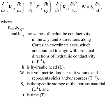 (1)
(1)
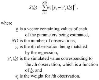 (2)
(2)
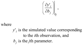 (3)
(3)
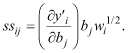 (4)
(4)
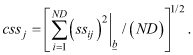 (5)
(5)
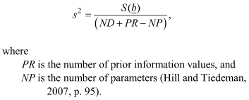 (6)
(6)