Error Analysis

Single Beam

The single-beam data were imported into ArcGIS, and a Python script was used to evaluate elevation differences at the intersection of trackline crossings. The script calculates the elevation difference between points at each intersection using an inverse distance weighting equation. Elevation values at line crossings should not differ by more than the combined instrument acquisition error (per manufacturer specified accuracies, tables 2-3). GPS cycle slips, stormy weather conditions, and rough sea surface conditions can contribute to poor data quality. If discrepancies that exceed the acceptable error threshold were found, then the line in error was either statically adjusted or removed. A line in error constitutes one or more of the following: (1) a segment where several crossings are incomparable, (2) a known equipment problem, or (3) known bad GPS data identified in the post-processing steps. For this dataset, elevation differences at 827 crossings were within ± 0.30 m, which accounts for 87 percent of the crossings. Only 5 percent were greater than ± 0.50 m.

Interferometric Swath

The stated horizontal accuracy of the Marinestar HP navigation subscription used during swath bathymetry acquisition is ± 10 centimeters (cm) horizontally and ± 15 cm vertically. The Coda Octopus F190R IMU integrates the Marinestar HP position with motion, measures vessel velocity (± 0.014 m/s), roll (± 0.025 degrees), pitch (± 0.025 degrees), heading (2 m baseline—0.5 cm), and heave (5 cm or 5 percent on-line) (table 6). The vertical accuracy for the SWATHplus-H system varies with depth and across track range. At maximum swath width the across track resolution can be within 1 cm depending upon water conditions and bottom type (table 7). Sound velocity captured in real-time at the transducer head was collected by a Valeport Mini SVS with a stated maximum error of ± 0.017 m/s (table 8). Sound velocity profile cast data tables were also applied to the swath data based on time, water depth, and spatial representation during the survey. The SVP data was captured with a Valeport Mini SVP with stated accuracy of ± 0.02 m/s (table 5).

Vertical Transformation

In addition to positional accuracies inherent for different datums (for example, NAD83, σ = 2.0 cm; NAVD88, σ = 5.0 cm; Mean Lower Low Water, MLLW, σ = 1.6 cm), error is introduced every time the data is transformed between datums. The transformation from ellipsoid height (ITRF00 for SBB and ITRF08 for IFB) to orthometric height (NAVD88) is σ = 7.0 cm, and the maximum cumulative uncertainty (quantified by standard deviation) introduced when transforming from ellipsoid height to orthometric height to a tidal datum (for example, MLLW) is 17.1 cm for eastern Louisiana (http://vdatum.noaa.gov/docs/est_uncertainties.html).

Digital Elevation Model

A comparison of the DEM versus the sounding (x,y,z point data) was performed to evaluate how well the DEM represented the original sounding data quantitatively and spatially. This was done by comparing the cell node values of the DEM surface to the final processed x,y,z point data using the Esri ArcGIS Spatial Analyst “extract values to points” tool. This produced a set of elevation differences between the gridded surface and the input data from which the root mean square error (RMS) was calculated using the following equation:

There are a total of 3,712,480 samples and the RMS of all points is 0.157 m. The differences between the point dataset and the extracted DEM values were color coded in order to visually evaluate differences (fig. 12). This comparison demonstrates how well the model surface represents the original sounding and sample data. The interpolated DEM resolution was constrained by a 50-m cell size. Trackline spacing varied depending on the survey method. The SBB tracklines were 100 m apart, and the IFB trackline spacing was 50 m in shallow water and extended to 250 m based upon swath width coverage in deeper water (fig. 12).

How well the DEM represents the data depends on how well the chosen DEM resolution compares to sounding distribution. In this example there may be hundreds of samples in a 50-m by 50-m cell; however, they are only represented on the surface by a single cell value. Therefore, in cases where terrain slope is high, the gridding formula reduces the actual variability in the sample data. This sacrifice is necessary when creating continuous surfaces over bathymetric datasets where trackline spacing did not allow for overlap. Finlayson and others (2011), Fregoso and others (2008), and Foxgrover and others (2004) also reported difficulty with gridding over steep slopes. The percent coverage of swath sample data relative to the elevation model area is approximately 28 percent, encompassing 22 km².

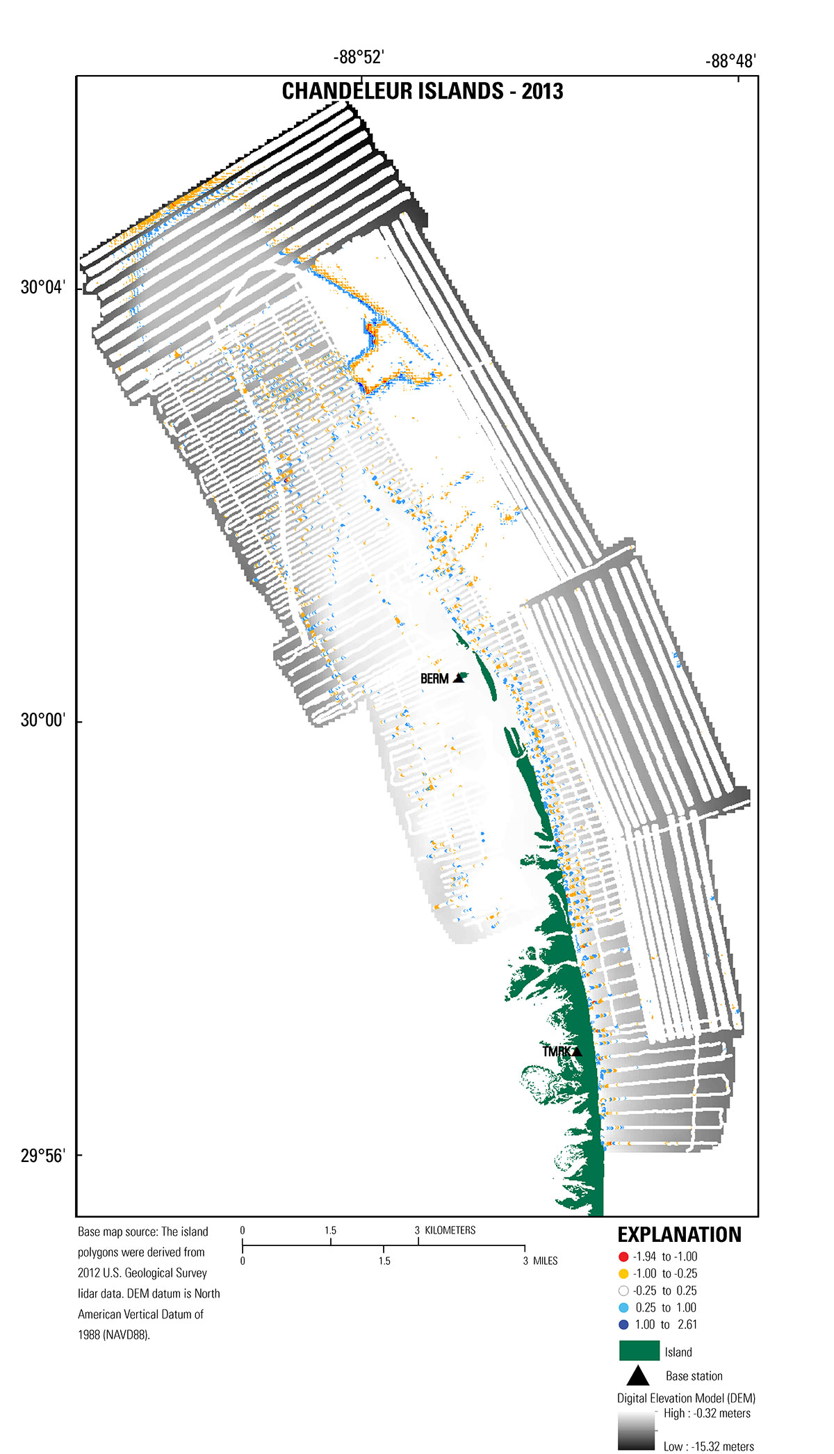Figure 12. Map showing error values (white circles) overlain upon the bathymetry grid (DEM), representing the difference between the bathymetry grid and each sample point (for positive values, the grid is deeper than the soundings; for negative values, the grid is shallower than soundings). White circles represent error of ± 0.25 meters. The island area extent is derived from U.S. Geological Survey light detection and ranging (lidar) collected in 2012, (Guy and others, 2014). [Click to enlarge]