Figure 3.1.  Photographs of the RV Connecticut (top) and the RV Ocean Explorer, both used for mapping surveys in this project. Click on figure for large image.

Figure 3.2.  Map showing tracklines of geophysical data in the nearshore area (red) and offshore area (green). USGS, U.S. Geological Survey; SAIC, Science Applications International Corporation. Click on figure for larger image.

Figure 3.3.  Map showing shaded-relief topography of seafloor offshore of northeastern Massachusetts between Cape Ann and Salisbury Beach. Coloring and bathymetric contours represent depths in meters, relative to the local mean lower low water (MLLW) datum. Click on figure for larger image.

Figure 3.4.  Map showing acoustic-backscatter intensity offshore of northeastern Massachusetts between Cape Ann and Salisbury Beach.  Backscatter intensity is an acoustic measure of the hardness and roughness of the seafloor.  In general, higher values (light tones) represent rock, boulders, cobbles, gravel, and coarse sand.  Lower values (dark tones) generally represent fine sand and muddy sediment.  Offshore data (green dashed outline) were collected by SAIC in 2004 and nearshore data (red dashed outline) were collected by USGS in 2005. Click on figure for larger image.

Figure 3.5.  Map showing the isopach of total sediment thickness (all sediment that overlies bedrock).  Small, isolated exposures of bedrock (dark gray shading) are covered with sediment less than 0.5 m thick.  Sediment-thickness values were interpreted from closely spaced seismic-reflection profiles.  In the nearshore area, measured values were used to generate an interpolated grid, but in the offshore area, they are only displayed as discrete points along the widely spaced tracklines. Click on figure for larger image.

Figure 3.6.  Map showing the thickness of sandy Holocene sediment (mobile sediment that overlies the transgressive unconformity).  Deposits thicker than 5 m are adjacent to the mouth of the Merrimack River and within Ipswich Bay.  Extensive areas offshore of central Plum Island and Salisbury Beach are covered by deposits thinner than 0.5 m.  Sediment-thickness values were interpreted from closely spaced seismic-reflection profiles.  In the nearshore area, measured values were used to generate an interpolated grid but, in the offshore area, the values are only displayed as discrete points along the widely spaced tracklines. Click on figure for larger image.

Figure 3.7.  Map showing the elevation of the transgressive unconformity, a gently sloping erosional surface that is etched into Pleistocene sediment.  Although locally buried by Holocene marine sediment up to 9 m thick, the unconformity is exposed at the seafloor in many locations.  Elevations of the transgressive unconformity were calculated by subtracting measured values of Holocene sediment thickness (fig. 3.6) from the combined bathymetric grid (fig. 3.3).  In the nearshore area, elevations were used to generate an interpolated grid, but in the offshore area, they are only displayed as discrete points along the widely spaced seismic-reflection tracklines.  Depths are relative to the local mean lower low water datum. Click on figure for larger image.

Figure 3.8.  Photograph of the SEABed Observation and Sampling System (SEABOSS) on the deck of the RV Connecticut.  Photographic data and sediment samples collected by the system were used to validate geophysical data and characterize seafloor environments. Click on figure for larger image.

Figure 3.9.  Map showing the locations of sediment samples and bottom photographs superimposed on a map of acoustic-backscatter intensity.  Each numbered circle indicates a station where bottom photographs, video, and/or samples were collected to validate interpretations of geophysical data. Click on figure for larger image.

• Field Program

• Bathymetry

• Acoustic Backscatter

• Seismic-Reflection Profiling

• Ground Validation

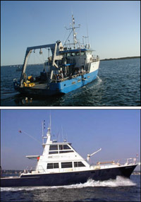
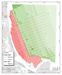
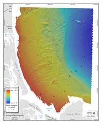
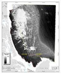
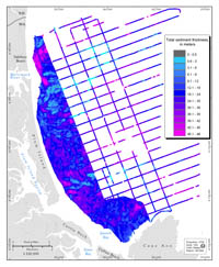
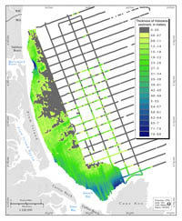
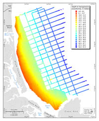
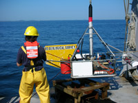
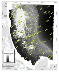
Field Program  

Acoustic data from interferometric and multibeam echo sounders (bathymetry and backscatter), a sidescan sonar (backscatter), and a chirp seismic-reflection profiler (subsurface stratigraphy and structure) were used to map approximately 325 km² of the inner continental shelf.  The mapping was conducted during two research cruises in 2004 and 2005, which respectively encompassed offshore and nearshore parts of the study area (fig. 1.1).  The convention of referring to the relatively deep offshore and shallow nearshore areas is used throughout this report because data in each area were acquired using different technologies and survey designs.  Methods used in the collection, processing, and analysis of the data are detailed in the following sections.  A full description of the data-acquisition and processing steps is available in the metadata that accompany this report.

The first cruise was conducted in the offshore part of the study area (water depths 25–92 m) by Science Applications International Corporation (SAIC) aboard the RV Ocean Explorer (fig. 3.1) between February 23 and March 23, 2004.  A multibeam echo sounder (MBES) was used to collect bathymetry and backscatter data, providing detailed imagery of 257 km² of the seafloor.

The second cruise was conducted in the nearshore part of the study area (water depths 2–30 m) by the USGS aboard the RV Connecticut (fig. 3.1) between September 8 and 20, 2005.  The survey included 9 days of geophysical data acquisition and 3 days of sampling.  Three acoustic systems (interferometric sonar, sidescan sonar, and chirp seismic-reflection profiler) were deployed simultaneously to collect bathymetry, backscatter, and subbottom data covering 68 km² of the seafloor.  After the geophysical survey was completed, the ship was equipped to collect sediment samples, bottom photographs, and video of the seafloor.

Bathymetry

In the offshore area, a RESON 8101 MBES operating at a frequency of 240 kHz was used to acquire bathymetric and backscatter data (SAIC, 2004).  The MBES was mounted on the keel of the ship.  A Position and Orientation System for Marine Vessels (POS/MV) was mounted on the vessel centerline just forward and above the MBES transducer and recorded vessel position and attitude data.  A Brooke Ocean Technology profiler measured sound velocity in the water column while the ship was underway.  Survey lines were run at an average speed of 9 knots in a NW–SE orientation (fig. 3.2). Depending on water depth, tracklines were spaced 50, 75, 100, and 125 m apart to achieve 100 percent coverage of the seafloor.  Data were processed by using Survey Analysis and Area Based Editor (SABER) software.  Tidal offsets, calculated using a discrete tidal zoning model and observations from the National Oceanic and Atmospheric Administration (NOAA) Tidal Station #8418150 at Portland, Maine (NOS CO-OPS , 2005), were used to reference the soundings to the local mean lower low water (MLLW) datum.  The bathymetric data have a vertical resolution of approximately 0.5 percent of water depth (SAIC, 2004).  The final bathymetric grid (fig. 3.3) was mapped at a resolution of 5 m/pixel.  Navigation for the offshore area utilized the signal from the U.S. Coast Guard Differential Global Positioning System.

In the nearshore area, bathymetry and backscatter data were collected with a SEA SwathPlus 234 kHz bathymetric system.  The interferometric sonar was mounted on a rigid pole on the starboard side of the ship with the transducers 3 m below the waterline.  A TSS DMS 2-05 inertial-motion unit was mounted directly above the sonar transducers and recorded vessel position and attitude data.  Sound-velocity profiles were collected approximately every 2 hours by a hand-casted Applied MicroSystems SV Plus Sound Velocimeter.  Survey lines were run at an average speed of 5 knots in a NW-SE orientation (fig. 3.2).  The lines were spaced 100 m apart to obtain 100 percent coverage of the seafloor.  Data were processed and gridded by using the CARIS Hydrographic Information Processing System (HIPS ver. 6.1).  The bathymetric data have a vertical resolution of approximately 1 percent of water depth.  The final bathymetric grid (fig. 3.3) was mapped at a resolution of 5 m/pixel.  Navigation for the nearshore area was based on a Real-Time Kinematic Global Positioning System (RTK-GPS).  The RTK-corrected GPS signal was sent to the ship once every second from a base station established by the USGS on land.  During post-processing, soundings were referenced to local MLLW by using orthometric to chart datum offsets obtained from NOAA Tidal Station #8440452 at the Parker River National Wildlife Refuge.

Acoustic Backscatter

In the offshore area, acoustic-backscatter and bathymetric data were collected simultaneously with the SAIC RESON MBES operating at a frequency of 240 kHz (SAIC, 2004; see Appendix 5).  The system has a 101-beam transducer that collects data in a continuous swath on either side of the vessel.  Depending on water depth, survey tracklines were spaced 50, 75, 100, and 125 m apart to achieve 100 percent coverage of the area.  The acquisition parameters for the MBES were maximized for collecting high-quality bathymetry instead of backscatter.  These acquisition parameters included power and gain changes that produced a striping effect in the backscatter mosaic.  The USGS reprocessed the raw MBES backscatter files in Generic Sensor Format (GSF) to minimize the power and gain artifacts by using a radiometric-correction technique developed by the Ocean Mapping Group and the University of New Brunswick (Beaudoin and others, 2002).

In the nearshore area, acoustic backscatter data were collected by using a Klein 3000 dual-frequency sidescan sonar (132/445 kHz) that was towed approximately 10 m off the bottom.  Backscatter intensity is an acoustic measure of relative hardness and roughness of the seafloor (fig. 3.4).  Data were acquired with Sonar Pro acquisition software and later corrected for beam angle and slant-range distortions by using Xsonar/Showimage as described in Danforth (1997).  The 132-khZ data from each survey line were mapped at 1 m/pixel resolution in geographic space in Xsonar, imported as raw image files to Geomatica GPC works (PCI Geomatica ver 8.2), and combined into a mosaic.  To correct for navigational uncertainties caused by towfish layback, the final mosaic was adjusted to match the bathymetry grid from the pole-mounted interferometric sonar.  The mosaic was exported out of PCI as a georeferenced Tagged Image File Format (TIFF) image for further analysis in ArcGIS.

Seismic-Reflection Profiling

Seismic-reflection profiles reveal the subsurface stratigraphy and geologic structure of the inner shelf.  Approximately 1100 km of high-resolution chirp seismic-reflection profiles (fig. 3.2) were collected by using an EdgeTech Geo-Star FSSB system and an SB-0512i towfish (0.5–12 kHz).  Delph Seismic+Plus acquisition software (Triton Elics International, Inc.) was used to control the topside unit and digitally log data in the SEG-Y rev. 1 standard format.  Data were acquired at a 0.25-s shot rate, a 9-ms pulse length, and a 0.5–6.0 kHz frequency sweep.  Trace lengths were adjusted between 100–200 ms to account for changes in water depth.  The SB-0512i was towed approximately 10 m astern and 3 m below the sea surface.  Navigation was obtained from the GPS receiver mounted above the interferometric sonar head.  On the basis of horizontal offsets between the towfish and GPS receiver, the positional accuracy was estimated to be ± 20 m.

Raw SEG-Y data were postprocessed with two Unix-based programs.  SIOSEIS (Scripps Institution of Oceanography) was used for amplitude-based seafloor picking and heave filtering, and Seismic Unix (Colorado School of Mines) was used to generate ASCII-formatted navigation files and JPEG compressed images of the profiles.  Navigation and processed SEG-Y data were imported into SeisWorks (Landmark Graphics, Inc.) for digital interpretation.  Reflections representing the tops of geologic units and unconformities were digitized to produce two-way travel time horizons.  A constant seismic velocity of 1500 m/s through water and sediment was used to convert travel time to distance.  Isopachs of total sediment thickness (i.e., sediment between bedrock and the seafloor) and Holocene sediment thickness (i.e., sediment overlying the transgressive unconformity) were exported at 30-shot intervals to produce ASCII point files containing shot position and associated thickness (figs. 3.5 and 3.6). 

Triangulated Irregular Network (TIN) surfaces were created from the ASCII point files and converted to regular grid (50 m/pixel) by using natural neighbors within ArcGIS 9.2.  An additional grid representing the transgressive unconformity (fig. 3.7) was generated by subtracting the isopach of Holocene sediment thickness from the gridded bathymetry.  Values from the gridded bathymetry were extracted at locations coincident to the points defining the Holocene sediment thickness.  Positive thickness values were then subtracted from the negative bathymetric values at each point, resulting in points representing the approximate elevation of the Holocene transgressive unconformity (relative to MLLW).  This point file was then used to generate a continuous, interpolated 50 m/pixel raster grid.  Utilization of isopach surfaces to generate these grids effectively removes the inherent static and time-varying vertical offsets associated with tidal fluctuations and deep towing of the SB-0512i towfish.

Ground Validation

In both the offshore and nearshore areas, geophysical data were validated with samples of surficial sediments and photographs of the seafloor.  A total of 87 locations were occupied for sampling and photography with the USGS SEABed Observation and Sampling System (SEABOSS; Valentine and others, 2000) (fig. 3.8).  Stations were selected to characterize backscatter transitions and broad areas of uniform backscatter intensity (fig. 3.9).  At each station, the SEABOSS was towed, or drifted with the current, over the bottom at speeds of 1 to 3 knots.  The recorded positions are actually the positions of the RTK-GPS antenna on the survey vessel, not the SEABOSS sampler, which was deployed from the stern of the vessel.  Because no layback or offset was applied to the recorded position, the estimated horizontal accuracy of the SEABOSS location is ± 40 m.  Continuous video was collected, usually for 5 to 15 minutes, and photographs were obtained from a still camera at all locations.  Sediment samples were usually collected at the end of each tow.  To prevent damage to sampling gear, no samples were collected in rocky, hardbottom areas.  The upper 2 cm of sediment were taken from the surface of the sediment sample for textural analysis.  All samples were analyzed for grain size by using standard procedures described in Poppe and others (2005).  Additional sediment-texture data are available for the region (Reid and others, 2005).  Although not included in this report, those data closely corroborated the bottom-type characterization in this study.