Figure 1.1.  Map showing the location of the survey areas offshore of northeastern Massachusetts between Cape Ann and Salisbury Beach.  The offshore area (green dashed outline) and nearshore area (red dashed outline)  were mapped in two separate cruises in 2004 and 2005, respectively. USGS, U.S. Geological Survey; SAIC, Science Applications International Corporation.

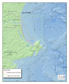Figure 1.2.  Late Quaternary relative sea-level curve for northeastern Massachusetts (modified from Oldale and others, 1993).  Over the last 14,500 years, relative sea level fell from a highstand of about +33 m to a lowstand of about –50 m, and then rose at varying rates to the present.  The large fluctuations in relative sea level drove regression (red shading) and transgression (green shading) of the shoreline across the inner continental shelf.  Dashed lines indicate uncertainty during the early to middle Holocene.  Note that the age scale changes at 8,000 years B.P.

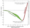Figure 1.3.  Air photograph of Plum Island and the mouth of the Merrimack River on the northeastern coast of Massachusetts.  A small drumlin (inset) anchors the southern end of the island.  Erosion of the drumlin provides sandy sediment to the barrier beach and has left behind a deposit of boulders on the beach and shoreface. (Photograph by Joseph Kelley, University of Maine, March 2005.)

Figure 3.1.  Photographs of the RV Connecticut (top) and the RV Ocean Explorer, both used for mapping surveys in this project.

Figure 3.2.  Map showing tracklines of geophysical data in the nearshore area (red) and offshore area (green). USGS, U.S. Geological Survey; SAIC, Science Applications International Corporation.

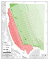Figure 3.3.  Map showing shaded-relief topography of seafloor offshore of northeastern Massachusetts between Cape Ann and Salisbury Beach. Coloring and bathymetric contours represent depths in meters, relative to the local mean lower low water (MLLW) datum.

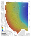Figure 3.4.  Map showing acoustic-backscatter intensity offshore of northeastern Massachusetts between Cape Ann and Salisbury Beach.  Backscatter intensity is an acoustic measure of the hardness and roughness of the seafloor.  In general, higher values (light tones) represent rock, boulders, cobbles, gravel, and coarse sand.  Lower values (dark tones) generally represent fine sand and muddy sediment.  Offshore data (green dashed outline) were collected by SAIC in 2004 and nearshore data (red dashed outline) were collected by USGS in 2005.

Figure 3.5.  Map showing the isopach of total sediment thickness (all sediment that overlies bedrock).  Small, isolated exposures of bedrock (dark gray shading) are covered with sediment less than 0.5 m thick.  Sediment-thickness values were interpreted from closely spaced seismic-reflection profiles.  In the nearshore area, measured values were used to generate an interpolated grid, but in the offshore area, they are only displayed as discrete points along the widely spaced tracklines. 

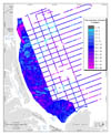Figure 3.6.  Map showing the thickness of sandy Holocene sediment (mobile sediment that overlies the transgressive unconformity).  Deposits thicker than 5 m are adjacent to the mouth of the Merrimack River and within Ipswich Bay.  Extensive areas offshore of central Plum Island and Salisbury Beach are covered by deposits thinner than 0.5 m.  Sediment-thickness values were interpreted from closely spaced seismic-reflection profiles.  In the nearshore area, measured values were used to generate an interpolated grid but, in the offshore area, the values are only displayed as discrete points along the widely spaced tracklines.

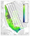Figure 3.7.  Map showing the elevation of the transgressive unconformity, a gently sloping erosional surface that is etched into Pleistocene sediment.  Although locally buried by Holocene marine sediment up to 9 m thick, the unconformity is exposed at the seafloor in many locations.  Elevations of the transgressive unconformity were calculated by subtracting measured values of Holocene sediment thickness (fig. 3.6) from the combined bathymetric grid (fig. 3.3).  In the nearshore area, elevations were used to generate an interpolated grid, but in the offshore area, they are only displayed as discrete points along the widely spaced seismic-reflection tracklines.  Depths are relative to the local mean lower low water datum.

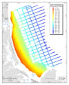Figure 3.8.  Photograph of the SEABed Observation and Sampling System (SEABOSS) on the deck of the RV Connecticut.  Photographic data and sediment samples collected by the system were used to validate geophysical data and characterize seafloor environments.

Figure 3.9.  Map showing the locations of sediment samples and bottom photographs superimposed on a map of acoustic-backscatter intensity.  Each numbered circle indicates a station where bottom photographs, video, and/or samples were collected to validate interpretations of geophysical data.

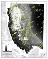Figure 4.1.  Interpretive geologic map showing five physiographic zones on the inner continental shelf, including Ebb-Tidal Delta, Nearshore Ramp, Outer Basin, Rocky Zone, and Shelf Valley.  Physiographic zones are superimposed on gray-scale, shaded-relief bathymetry except in areas adjacent to the shoreline in shallow water landward of the survey area.  See Section 4 – Interpretive Geologic Mapping for a detailed description of each zone.  Index boxes and profile lines show locations for other figures used in this report.

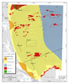Figure 4.2.  Maps showing bathymetry (upper left) and acoustic-backscatter intensity (upper right) in the south-central part of the survey area.  The eroded remnants of a large till deposit, probably a drumlin or moraine, represents a discrete Rocky Zone (RZ) surrounded by Nearshore Ramp (NR).  Bottom photographs A–C and the seismic-reflection profile (bottom) are indicated by yellow circles and a red line, respectively.  The distance across the bottom of the photographs is approximately 50 cm.  See Figure 4.1 for location.  NR = Nearshore Ramp; RZ = Rocky Zone.  A constant seismic velocity of 1500 m/s through water, sediment, and rock was used to convert from two-way travel time to depth.

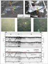Figure 4.3. Seismic-reflection profile across the inner continental shelf.  Stratified glacial-marine sediment rests on bedrock and is overlain by fluvial and deltaic deposits that formed during coastal regression and sea-level lowstand.  Seaward-dipping clinoforms (inset B) indicate progradation of the delta offshore into a deep, muddy basin.  The prominent transgressive unconformity (red line) is an erosional surface that caps the fluvial/deltaic sequence and grades to conformity below depths of about 50 m.  A seaward-thinning wedge of sediment, interpreted as estuarine in origin, underlies shallow parts of the inner shelf (inset A).  Holocene deposits of sandy marine sediment locally overlie the transgressive unconformity.  See Figure 4.1 for location.  A constant seismic velocity of 1500 m/s through water, sediment, and rock was used to convert from two-way travel time to depth.

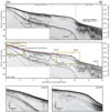Figure 4.4.  Maps showing bathymetry (upper left) and acoustic-backscatter intensity (upper right) in the northwestern part of the survey area.  A small Shelf Valley (SV) cuts through a large expanse of Rocky Zone (RZ), adjacent to the relatively smooth, sand- and gravel-covered surface of the Nearshore Ramp (NR).  Bottom photographs A–C and seismic-reflection profile (bottom) are indicated by yellow circles and a red line, respectively.  The distance across the bottom of the photographs is approximately 50 cm.  See Figure 4.1 for location.  A constant seismic velocity of 1500 m/s through water, sediment, and rock was used to convert from two-way travel time to depth.

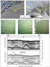Figure 4.5. Maps showing bathymetry (upper left) and acoustic-backscatter intensity (upper right) on the Nearshore Ramp (NR) in the central part of the survey area.  Parallel stripes that trend NW-SE in the backscatter data are artifacts of data collection.  Color coding on the depth profile (bottom) shows high backscatter (coarse sand and gravel) in the shallow depression and low backscatter (fine sand) on the adjacent, bathymetrically higher areas.  Bottom photographs (A and B) collected on opposite sides of the backscatter transition illustrate the different grain sizes that produce the changes in intensity.  The distance across the bottom of the photographs is approximately 50 cm.  See Figure 4.1 for location.

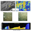Figure 4.6.  Maps showing bathymetry (upper left) and acoustic-backscatter intensity (upper right) in the northeastern part of the survey area.  Parallel stripes that trend NW-SE in the backscatter data are artifacts of data collection.  Isolated Rocky Zones (RZ) are surrounded by the uniformly flat, muddy seafloor of the Outer Basin (OB).  Bottom photographs A–F are indicated by yellow circles.  The distance across the bottom of the photographs is approximately 50 cm.  See Figure 4.1 for location.

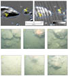Figure 4.7.  Graph showing the relationship between mean backscatter values (DN = digital number) and mean grain size for 14 bottom samples collected in the nearshore area.  Sediment in areas of relatively high backscatter (values greater than 45) consists of coarse sand.  Sediment in areas of relatively low backscatter (values less than 45) primarily consists of fine sand.  No samples of medium sand (gray box) were collected. 

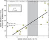Figure 4.8.  Maps of the nearshore area showing the three inputs to the quantitative bottom classification: (A) water depth, (B) bathymetric slope, and (C) acoustic-backscatter intensity.  Map D shows the predicted texture of surficial sediment in the area and the mean grain size of the 14 sediment samples represented by the graph in figure 4.7.  Appendix 4 describes the processing flow for the analysis, input data, and functions used to generate this classification.

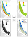Figure 4.9.  Ternary diagrams depicting texture of surficial sediment in samples collected from the survey area.  Apexes of the diagrams represent 100 percent of the labeled textural component (i.e., gravel, sand, silt, and/or clay).  The upper diagram depicts 45 samples that lack gravel; the lower diagram depicts 34 samples that contain at least 0.5 percent gravel.  See table 4.2 for additional information on these samples.

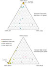Figure 4.10.  Seismic-reflection profile showing three small channels cut into glacial-marine sediment in the central part of the study area.  The transgressive unconformity (red line) is eroded into the upper surface of fluvial deposits and locally overlain by a sheet of sandy marine sediment generally less than 1 m thick.  See Figure 4.3 for location.  A constant seismic velocity of 1500 m/s through water, sediment, and rock was used to convert from two-way travel time to depth.

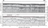Figure 4.11.  Seismic-reflection profile showing a broad channel cut into fluvial and glacial-marine sediment in the southern part of the study area.  The well-stratified sediment that fills the channel is interpreted as estuarine sediment.  The transgressive unconformity (red line) is overlain by 5 to 6 m of sandy marine sediment, which is among the thickest Holocene deposits in the region.  See Figure 4.3 for location.  A constant seismic velocity of 1500 m/s through water, sediment, and rock was used to convert from two-way travel time to depth.

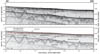Figure 4.12.  A four-phase conceptual model showing evolution of the northeastern Massachusetts coast and inner shelf as interpreted from geologic mapping.  Schematic diagrams depict the general configuration of coastal landforms and stratigraphic units.  Timing and elevation of relative sea level (RSL) are based on published reports and our best estimates.  Each panel includes an outline of Plum Island in its present location.  Phase 1: Late Pleistocene glaciers retreat across the isostatically depressed landscape, and leave behind drumlins and other till deposits.  RSL is about 33 m higher than present.  Thick glacial-marine sediment blankets high-relief bedrock.  Phase 2: With crustal rebound, RSL falls to a lowstand of about –50 m depth.  Braided streams flow across the emergent landscape and deposit a broad, relatively thin sheet of fluvial sand and gravel.  A large delta forms at the lowstand shoreline about 10 km seaward of the present coast.  Muddy marine sediment accumulates in deeper water.  Phase 3: Early Holocene RSL rises to 20 to 30 m.  Shoreline migration reworks the upper surface of the lowstand delta.  Erosion produces a transgressive unconformity that is overlain by thin, discontinuous deposits of sandy marine sediment.  A barrier island/spit, which is pinned to eroding drumlins, probably has formed seaward of Plum Island.  Phase 4: RSL rise continues and the barrier/spit system migrates to its present location.  Rocky Zone represents ledge or eroded remnants of drumlins.  Nearshore Ramp represents the modified, gently sloping delta top.  Ebb-Tidal Deltas form seaward of inlets.  Channel-fill deposits are interpreted as estuarine sediment that accumulated in a back-barrier setting.  Thick muddy sediment is preserved in the Outer Basin below the depth of RSL lowstand.  (Photograph in panel 4 by Joseph Kelley, University of Maine, March 2005.)