Click on figure for larger image.

Figure 2. Continuous resistivity profile (CRP) streamer coiled on the deck of the survey vessel during transit. Foam flotation is attached to the cable between each electrode. Photo by John Bratton, USGS-GD-WHCMSC.

Figure 3.: Continuous resistivity profile (CRP) streamer being towed behind the survey vessel. Photo by John Bratton, USGS-GD-WHCMSC.

Figure 4. The Continuous resistivity profile (CRP) data acquisition system included the AGI SuperSting R8 Resistivity Meter (foreground) and the display screen of the Lowrance GPS-enabled fathometer. Photo by John Bratton, USGS-GD-WHCMSC.

Figure 5. Seismic source and receiver attached to the port side of the survey vessel and pivoted out of the water during transit. The instrument shown on the right side of the blue bucket on the deck was used to measure the conductivity and temperature of surface water, which was pumped continuously into the bucket during surveying. Photo by John Bratton, USGS-GD-WHCMSC.

Figure 6. Seismic source and receiver deployed from the side of the vessel during surveying. Photo by John Bratton, USGS-GD-WHCMSC.

Figure 7. The seismic data acquisition system included a real-time data display and processors shown here. Photo by John Bratton, USGS-GD-WHCMSC.

Data collection and processing methods are described here for continuous resistivity profile (CRP) data and the Chirp seismic-reflection data collected aboard the R/V Kerhin from September 6 to September 8, 2006 (Julian day 249 to Julian day 251) in the Potomac River Estuary. These data were collected simultaneously except for one brief time period on September 6 when the seismic acquisition system was inoperable.

Continuous Resistivity Profiling (CRP)

CRP data were collected in the Potomac River Estuary in 2006, as summarized in the table below, using methods similar to those described by Cross and others (2006 and 2008).

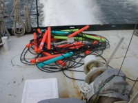
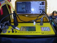
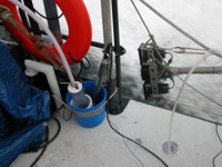
Data were collected using an Advanced Geosciences, Inc. (AGI) system (figs. 2 and 3). The AGI cable is a 100-meter streamer with an 11-electrode array, with electrodes spaced 10 meters apart. The two source electrodes are graphite, while the nine receiver electrodes are stainless steel. Foam flotation is attached to the cable between each electrode to keep the cable at or near the surface, while allowing the electrode to hang a little below the water surface and helping to keep the electrode in the water in mildly choppy seas. The depth of penetration of this system is approximately 20 percent of the towed cable length. A dipole-dipole configuration was used for the data collection in which two fixed-current electrodes were assigned, and voltage potentials were then measured between electrode pairs in the remaining nine electrodes.

Among other applications, CRP surveys are conducted to determine electrical resistivity of the subsurface in order to distinguish fresh from saline groundwater in shallow sedimentary units over large areas (Manheim and others, 2004; Cross and others, 2006, 2008). The initial values recorded by the system are measured apparent resistivity values. A two-dimensional (2D) resistivity model takes into account resistivity changes in the vertical and horizontal direction along a survey line, while assuming resistivity remains constant perpendicular to the survey line (Loke, 2000). The apparent resistivity data undergo an inversion process, which produces a resistivity profile that is most consistent with the measured values. EarthImager 2D inversion software divides the subsurface into a number of rectangular blocks. The resistivity of each of these blocks is determined, creating an apparent resistivity pseudosection that is consistent with the measured apparent resistivity values. By constraining the model with the water-depth profile, where water thickness (depth) and resistivity are known from field measurements, a more accurate subsurface-resistivity profile can be generated. Processing parameters can be used to further constrain the modeling. The data, both raw and processed, including metadata compliant with Federal Geographic Data Committee (FGDC) standards, can be accessed through the Data Catalog page.

The shipboard control and logging system used for the data collection of the resistivity streamer was an AGI SuperSting R8 Marine Resistivity Meter (fig. 4). Current was injected into the water/sediment system approximately every 3 seconds through the source electrode pair at the front end of the streamer, and 8 apparent resistivity values representing 8 depth levels were recorded for each current injection. A Lowrance LMS-480M GPS with an LGD-2000 GPS antenna and a 200-kiloherz fathometer transducer with a temperature sensor were also attached to the system in order to acquire navigation and depth.

At the end of each day of data acquisition, the CRP and navigation/depth data were downloaded from the SuperSting system using a laptop running AGI's Marine Log Manager software. The data were then transferred to a processing computer in order to check the quality of the navigation data and process the CRP data using AGI's Marine Log Manager and EarthImager 2D software packages. The Marine Log Manager software was used to merge the navigation file (file extension GPS) with the raw resistivity data (file extension STG), resulting in a linearized resistivity file (STG file extension) and a file containing the depth and temperature data when available (DEP file extension). These files are used as input to AGI's EarthImager 2D software for data processing.

The DEP files can be modified to include the water resistivity value measured at the time of surveying. A second instrument used during this survey, a YSI, Inc. 600 XLM datasonde,  simultaneously collected surface water conductivity and temperature data (fig. 5). These data were used to calculate the average water resistivity value over an individual CRP survey line. This information was then added to the DEP file used in processing the data.

EarthImager 2D version 1.9.9 was used to process the data files (STG and DEP) using the supplied CRP saltwater processing parameters which have minimum and maximum allowable resistance and voltages appropriate for the marine environment. The EarthImager 2D CRP module is specifically designed to process large amounts of continuous resistivity data, as are typically acquired during marine surveys. The strategy for data processing could be described as a "divide-and-conquer" method, in which the long section of a single collection file is divided into many subsections. These subsections are individually inverted, and the processing culminates by assembling the individual sections into a single profile (Advanced Geosciences Inc., 2005). The output files from all of these steps are saved into an individual folder. For the purposes of this report, the linearized STG and DEP files used as input for the processing were saved, as well as three file types generated during processing. These include:

1. JPEG images of the complete resistivity profile. Both long and short versions are available for each line.
2. Text files of the processed resistivity data. These include XYZ files in which X = distance along line, Y = depth, and Z = resistivity value. Also included are LLT files, which contain longitude, latitude, depth, and resistivity values.
3. A file with the INI extension containing the processing parameters used. This INI file can be loaded prior to subsequent file processing to ensure that the same parameters are used for all files or to verify the processing parameters used.

The JPEG images resulting from the EarthImager 2D processing were saved with the default color scale. This color scale ranges from blues to reds with reds representing the higher resistivity values corresponding to fresher (less saline) groundwater. The color scale within each image is maximized for the range of resistivity values from that survey line.

In addition, in order to more easily compare different resistivity profiles, MATLAB software was used to combine the XYZ and DEP files to generate JPEG images with a common color scale for all survey line files. Within these images, the polarity of the color scheme is the same as that of the EarthImager 2D JPEGs, in that the colors range from blue to red with reds indicating higher resistivity values. MATLAB software was also used to plot the data in an attempt to display the JPEG images with a common vertical and horizontal distance scale. Rounding errors in figure size scaling prevent exact reproducibility of scale in the horizontal direction for the images.

Both the EarthImager 2D and the MATLAB JPEG images can be accessed from the Resistivity Profile Previews page.

MATLAB was also used to remove the water-column resistivity data from the XYZ files based on the water depth data in the DEP data files. Both the DEP and XYZ data were interpolated within MATLAB in order to extract a resistivity value for the sediment/water interface. The interpolated value, along with the measured values within the sediment, was exported to the modified XYZ data file. All of the CRP lines were processed, and the results were combined into a single shapefile (mrg2006_allxyz) available from the Data Catalog page.

Finally, a Visual Basic 6 program was written to combine the linearized STG file with the DEP file from each survey line to create a data file in RES2DINV format for users of that software package. These files are also available from the Data Catalog page.

Seismic-Reflection Profiles

Chirp sub-bottom profiles were collected using a Knudsen Engineering Limited (KEL) 1600 Universal Serial Bus (USB) system with a peak frequency of 3.5 kilohertz. Two Massa 3.5-kiloherz transducers were pole-mounted (fig. 5 and fig. 6) over the port side of the ship. The transducer was 0.7 meters below the water surface and there was a 2-meter horizontal offset from the DGPS antenna. Vertical draft and horizontal offset corrections were not applied to the raw data. The system was fired five times per second with a trace length of 41 milliseconds. The sub-bottom data were recorded in Knudsen Engineering Binary (KEB) format, and shot point and time were logged as Knudsen Engineering ASCII (KEA) files using KEL SounderSuite software (fig. 7). The navigation was not logged to KEB or KEA files for Julian days 149 and 150 due to a problem with the SounderSuite software. This problem was resolved on Julian day 151 with an updated version of SounderSuite. Time of day in the KEB and KEA files was derived from system time on the acquisition computer. System time on the KEL and HYPACK navigation system was synchronized to GPS time with a timeserver.

KEB files were converted to KEL SEG-Y (Norris and Faichney, 2002) format using KEL PostSurvey software. KEB, KEA, and SEG-Y files were transferred to an external hard drive and copied to a Macintosh PowerBook for processing. The KEL SEG-Y data were match filtered but not in typical instantaneous (envelope) format.  SIOSEIS (SIOSEIS, 2006) software was used to convert the trace data to envelope data, which were then saved in SEG-Y rev. 1 standard format. Seismic Unix (Stockwell and Cohen, 2008) was used to read the SEG-Y files, apply and automatic gain control (AGC) with a 7.5-millisecond window, and create JPEG plots of the trace data.

Shot point navigation was derived by merging shot point and time with navigation fixes from HYPACK navigation. The HYPACK navigation data were parsed to output time of day and UTM Zone 18 eastings and northings. These data were merged with shot-point number, Julian day, and time of day extracted from the SEG-Y trace headers using the Unix Join command. This produced a shot-point navigation file with fixes every 1 second (five shots). Julian day 151 was processed the same way even though position was recorded in the trace headers.

JPEG images of these profiles can be accessed from the Profiles Previews page for the seismic data.