Open-File Report 2011-1039
MethodsData collection and processing methods are described here for continuous resistivity profiling (CRP) data and chirp seismic-reflection data collected aboard the R/V Knob in Indian River Bay, Delaware. The CRP data were collected from April 13 to April 15, 2010 (Julian day 103 to Julian day 105), while chirp seismic-reflection data were only collected on April 13. Continuous Resistivity Profiling (CRP)CRP data were collected in Indian River Bay in 2010 using methods similar to those described by Cross and others (2010, 2013). In this study, data were collected with a 50-m resistivity streamer for 145 km. Table 1 summarizes the processed CRP data collection.
Data were collected using an Advanced Geosciences, Inc. (AGI) SuperSting R8 Marine resistivity system (figs. 2 and 3). The AGI cable used on this survey is a 50-m streamer with an 11-electrode array with electrodes spaced 5 m apart. The two source electrodes are graphite, whereas the nine receiver electrodes are stainless steel. Foam flotation was attached to the cable between each electrode to keep the cable at or near the surface while allowing the electrodes to hang a little below the water surface, helping to keep the electrodes in the water in mildly choppy seas. The depth of penetration of this system is approximately 25 percent of the towed cable length. A dipole-dipole configuration was used for the data collection in which two fixed-current electrodes were assigned, and voltage potentials were then measured between electrode pairs in the remaining nine electrodes. Among other applications, CRP surveys are conducted to determine electrical resistivity of the subsurface in order to distinguish fresh from saline groundwater in shallow sedimentary units over large areas (Manheim and others, 2004; Cross and others, 2010, 2013). The initial values recorded by the system are measured apparent resistivity values. A two-dimensional (2D) resistivity model takes into account resistivity changes in the vertical and horizontal directions along a survey line, while assuming resistivity remains constant perpendicular to the survey line (Loke, 2000). The apparent resistivity data undergo an inversion process that produces a resistivity profile most consistent with the measured values. EarthImager 2D inversion software divides the subsurface into a number of rectangular blocks. The resistivity of each of these blocks is determined, creating an apparent resistivity pseudosection that is consistent with the measured apparent resistivity values. By constraining the model with the water-depth profile, where water thickness (depth) and resistivity are known from field measurements, a more accurate subsurface resistivity profile can be generated. Processing parameters, such as the type of inversion process, number of iterations, and amount of roll-along data overlap, can be used to further constrain the modeling. The raw and processed data, including metadata compliant with Federal Geographic Data Committee (FGDC) standards, can be accessed through the Data Catalog page. The metadata files give full details on the parameters used to process the data. The shipboard control and logging system used for the data collection of the resistivity streamer was an AGI SuperSting R8 Marine resistivity meter (fig. 3). Current was injected into the water/sediment system approximately every 3 seconds through the source electrode pair at the front end of the streamer, and eight apparent resistivity values representing eight depth levels were recorded for each current injection. A Lowrance LMS-480M Global Positioning System (GPS) with an LGD-2000 GPS antenna and a 200-kilohertz fathometer transducer with a temperature sensor were also attached to the system to acquire navigation and measure water depth. At the end of each day of data acquisition, the CRP and navigation/depth data were downloaded from the SuperSting system to a laptop computer running AGI's Marine Log Manager software. The data were then transferred to a processing computer to check the quality of the navigation data and process the CRP data using AGI's Marine Log Manager and EarthImager 2D software packages. The Marine Log Manager software was used to merge the navigation file (file extension GPS) with the raw resistivity data (file extension STG), resulting in a linearized resistivity file (file extension STG) and a file containing the depth and temperature data when available (file extension DEP). These files are used as input to AGI's EarthImager 2D software for data processing. The DEP files can be modified to include the water resistivity value measured at the time of surveying. Another instrument used during this survey, a YSI, Inc. 600 XLM data sonde, simultaneously collected surface-water conductivity and temperature data. These data were used to calculate the average water resistivity value over an individual CRP survey line. This information was then added to the DEP file used in processing the data. The average water resistivity value was appropriate for processing most of the survey lines. However, several survey lines extended from near the inlet in the east all the way to the fresher water sources in the west. These lines (L1F7, L4F1, L8F1, L9F3, L19F2, L20F2, and L38F1) were also processed using a water conductivity file (file extension CON) that incorporates the water resistivity variation over the length of the line. The resistivity values in the CON files were calculated from water conductivity values recorded with the YSI sensor based on the inverse relationship between the two measurements. EarthImager 2D version 2.2.8 was used to process the data files (STG and DEP in all cases and STG and CON for some of the lines) using the supplied CRP saltwater processing parameters, which have minimum and maximum allowable resistance and voltages appropriate for the marine environment. The EarthImager 2D CRP module is specifically designed to process large amounts of continuous resistivity data, as are typically acquired during marine surveys. The strategy the software uses for data processing could be described as a "divide-and-conquer" method in which the long section of a single collection file is divided into many subsections. These subsections are individually inverted, and the processing culminates by assembling the individual sections into a single profile (Advanced Geosciences, Inc., 2005). The output files from all of these steps are saved into an individual folder. For the purposes of this report, the linearized STG and DEP files used as input for the processing were saved, as well as three file types generated during processing. When continuously measured water conductivity files were used, the linearized STG and CON files were saved, as well as three file types generated during processing. These three file types common to both methods of processing include:
The JPEG images resulting from the EarthImager 2D processing were saved with the default color scale. This color scale ranges from blues to reds with reds representing the high resistivity values corresponding to fresher (less saline) groundwater. The color scale within each image is maximized for the range of resistivity values from that survey line. In addition, to more easily compare resistivity profiles, the MathWorks, Inc. MATLAB software was used to combine the XYZ and DEP files to generate JPEG images with a common color scale for all survey line files. Within these images, the polarity of the color scheme is the same as that of the EarthImager 2D JPEGs, in that the colors range from blue to red with reds indicating high resistivity values. MATLAB was also used to plot the data in an attempt to display the JPEG images with a common vertical and horizontal distance scale. Rounding errors in figure size scaling prevent exact reproducibility of scale in the horizontal direction for the images. Both the EarthImager 2D and the MATLAB JPEG images can be accessed from the Resistivity Profile Previews pages. MATLAB was also used to remove the water-column resistivity data from the XYZ files based on the water depth data in the DEP data files. Both the DEP and XYZ data were interpolated within MATLAB in order to extract a resistivity value for the sediment/water interface. The interpolated value, along with the measured values within the sediment, was exported to the modified XYZ data file. All of the CRP lines were processed, and the results were combined into single shapefiles based on survey day. A separate shapefile exists for the CRP lines processed with a continuously measured water conductivity value. All of these files are available from the Data Catalog page. Finally, a Visual Basic 6 program was written to combine the linearized STG file with the DEP file from each survey line to create a data file in RES2DINV format for users of that software package. These files are available from the Data Catalog page. Chirp Seismic-Reflection ProfilesChirp sub-bottom profiles were collected using an EdgeTech portable 3100 sub-bottom profiling system and SB-424 chirp towfish (fig. 4) operating at a 4- to 24-kilohertz pulse bandwidth and a 2-millisecond pulse. The towfish containing the system transmitters and receiving hydrophones was deployed from a short line attached to a cleat on the starboard side of the boat and was towed approximately 0.5 m below the water surface. EdgeTech Discover acquisition software was used to record the data in SEG-Y format (Norris and Faichney, 2002). Navigation was supplied by a Lowrance GPS system with the antenna mounted topside on a pole coincident with the tow position of the chirp transducer. The navigation was written to the header of the SEG-Y files in arc-second format. Vertical draft offset corrections were not applied to the raw data. The system fired four to six times per second with a trace length of 133 milliseconds, a sample interval of 23 microseconds, and 5,788 samples per trace. Seismic Unix (Stockwell and Cohen, 2008) was used to read the SEG-Y files, apply an automatic gain control, and create JPEG plots of the trace data. Due to problems with the acquisition system, seismic-reflection data were only collected on the first day of surveying. JPEG images of these profiles can be accessed from the Seismic Profiles Previews page. These files, as well as the SEG-Y data files, are also available from the Data Catalog page.
|

![]() U.S. Department of the Interior |
U.S. Geological Survey
U.S. Department of the Interior |
U.S. Geological Survey
URL: http://pubsdata.usgs.gov/pubs/of/2011/1039/html/ofr2011-1039-methods.html
Page Contact Information: GS Pubs Web Contact
Page Last Modified: Thursday, 24-Jul-2014 14:45:27 EDT