Skip past header information
USGS - science for a changing world

U.S. Geological Survey Open-File Report 2011-1040

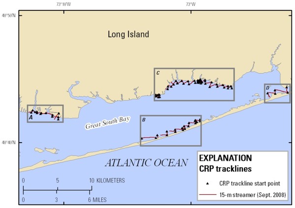
Continuous Resistivity Profiling Data From Great South Bay, Long Island, New York


Continuous Resistivity Profile Previews—Sept. 2008—Area B

Skip past contents information

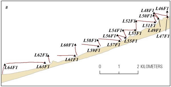
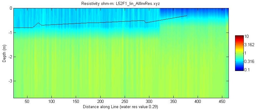
The table below contains previews of the 15-m streamer CRP data from area B processed using the average measured water resistivity value (WRES) of 0.29 ohm-m. The EarthImager 2D JPEG and MATLAB JPEG images of each processed file are presented. In addition, the area B trackline map below is a "clickable" map. By clicking on a line name, a new window will open with the processed images from that particular line segment. This new window will contain a reduced version of the EarthImager 2D JPEG image (short version) as well as the MATLAB JPEG image. The beginning of each line is marked with a triangle on the map. The left side of the associated JPEG image represents the beginning of the line and corresponds to the triangle on the map.

Trackline map of processed 15-m streamer CRP lines collected in Great South Bay in September, 2008.

An enlarged portion of the trackline map of processed 15-m streamer CRP lines collected in Great South Bay in Area B September, 2008. Line names provide hotlinks to the JPEG profiles.

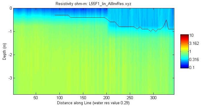
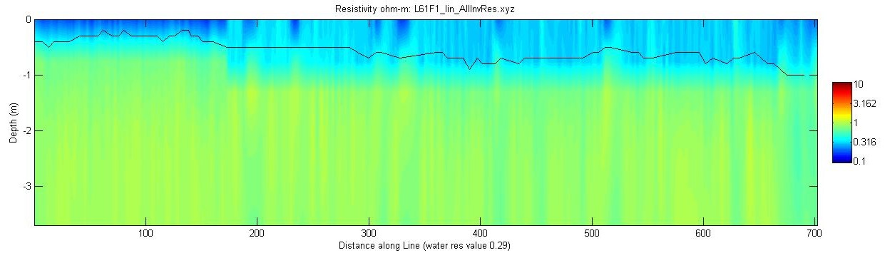
Preview of Profiles—Click individual images to see full-size JPEG images of the profile. For the EarthImager 2D versions, the long version of the profile is available. All of the profiles are available for download from the Data Catalog page.

In the EarthImager 2D version, the white line in the image represents the water depth as measured by the fathometer. In the MATLAB-generated JPEG images, the water depth is represented by a black line. The JPEG images resulting from the EarthImager 2D processing were saved with the default color scale generated by the software. This color scale ranges from blues to reds with reds representing the higher resistivity values corresponding to fresher (less saline) groundwater. Each individual image has the scale maximized for the range of resistivity values in that dataset. The MATLAB versions of the JPEG images use a common color scale for all the files to facilitate profile comparison. For these images, the polarity of the color scheme is the same as that of the EarthImager 2D JPEGs in that the colors range from blue to red with reds indicating higher resistivity values corresponding to fresher (less saline) groundwater. In the MATLAB version, the x axis represents distance along line in meters. The EarthImager 2D version x-axis units are latitude and longitude (position) along line. On the second day of surveying, the temperature information was available at times and included with the resistivity profile when available. The temperature information was available for all of the lines on the third day of surveying. On extremely short lines that did not require the roll-along processing, the temperature plot is not generated during EarthImager processing, and the x-axis units are distance along line in meters. Additionally, on these short lines the MATLAB image titles and x-axis labels are often truncated.


EarthImager version MATLAB version
Sept. 24, 2008: Line L46F1, WRES = 0.29
EarthImager thumbnail JPEG image of line 46 resistivity and temperature profile.
MATLAB thumbnail JPEG image of line 46 resistivity profile.
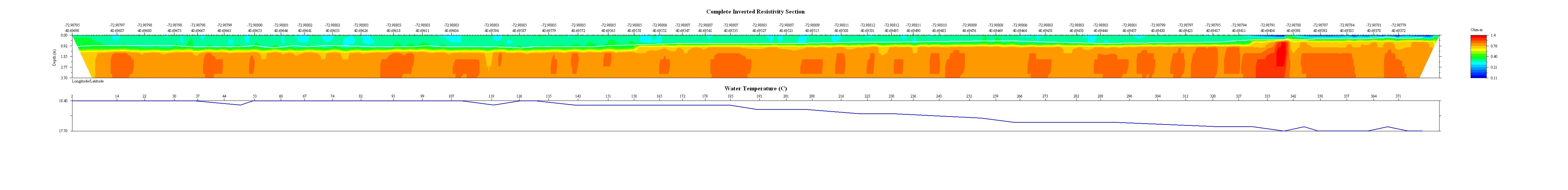
Sept. 24, 2008: Line L47F1, WRES = 0.29
EarthImager thumbnail JPEG image of line 47 resistivity and temperature profile.
MATLAB thumbnail JPEG image of line 47 resistivity profile.
Sept. 24, 2008: Line L48F1, WRES = 0.29
EarthImager thumbnail JPEG image of line 48 resistivity and temperature profile.
MATLAB thumbnail JPEG image of line 48 resistivity profile.
Sept. 24, 2008: Line L49F1, WRES = 0.29
EarthImager thumbnail JPEG image of line 49 resistivity and temperature profile.
MATLAB thumbnail JPEG image of line 49 resistivity profile.
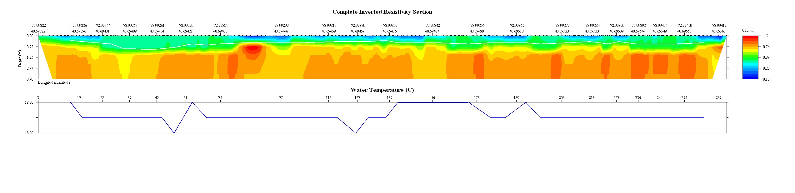
Sept. 24, 2008: Line L50F1, WRES = 0.29
EarthImager thumbnail JPEG image of line 50 resistivity and temperature profile.
MATLAB thumbnail JPEG image of line 50 resistivity profile.
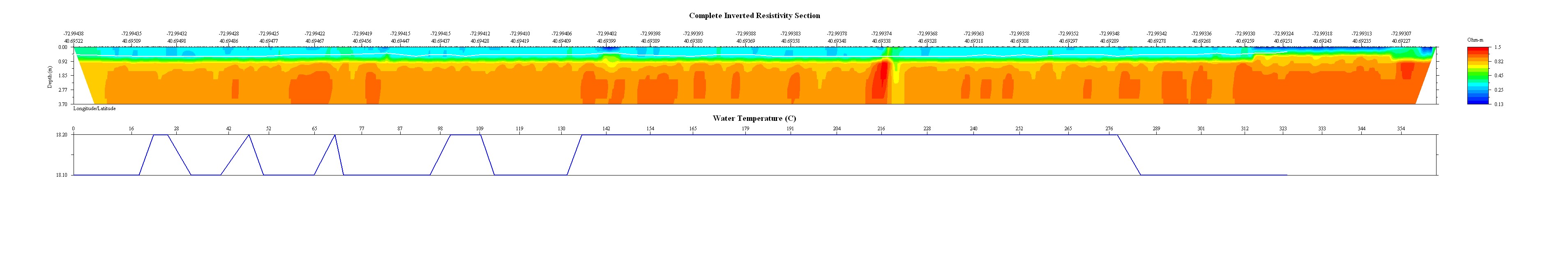
Sept. 24, 2008: Line L51F1, WRES = 0.29
EarthImager thumbnail JPEG image of line 51 resistivity and temperature profile.
MATLAB thumbnail JPEG image of line 51 resistivity profile.
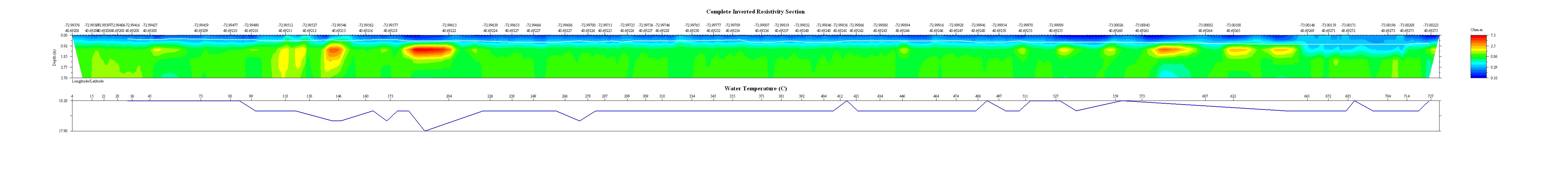
Sept. 24, 2008: Line L52F1, WRES = 0.29
EarthImager thumbnail JPEG image of line 52 resistivity and temperature profile.
MATLAB thumbnail JPEG image of line 52 resistivity profile.
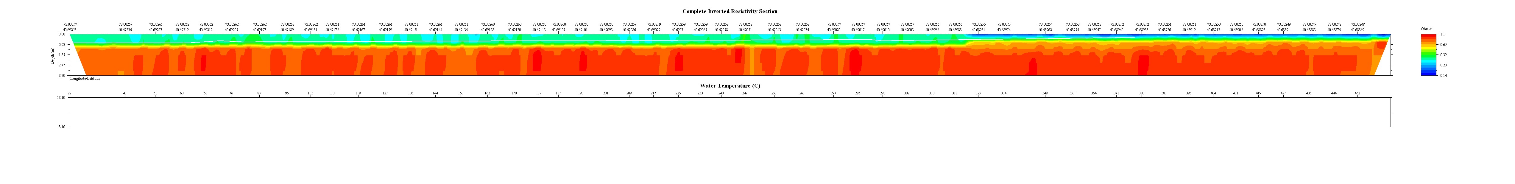
Sept. 24, 2008: Line L53F1, WRES = 0.29
EarthImager thumbnail JPEG image of line 53 resistivity and temperature profile.
MATLAB thumbnail JPEG image of line 53 resistivity profile.
Sept. 24, 2008: Line L54F1, WRES = 0.29
EarthImager thumbnail JPEG image of line 54 resistivity and temperature profile.
MATLAB thumbnail JPEG image of line 54 resistivity profile.
Sept. 24, 2008: Line L55F1, WRES = 0.29
EarthImager thumbnail JPEG image of line 55 resistivity and temperature profile.
MATLAB thumbnail JPEG image of line 55 resistivity profile.
Sept. 24, 2008: Line L56F1, WRES = 0.29
EarthImager thumbnail JPEG image of line 56 resistivity and temperature profile.
MATLAB thumbnail JPEG image of line 56 resistivity profile.
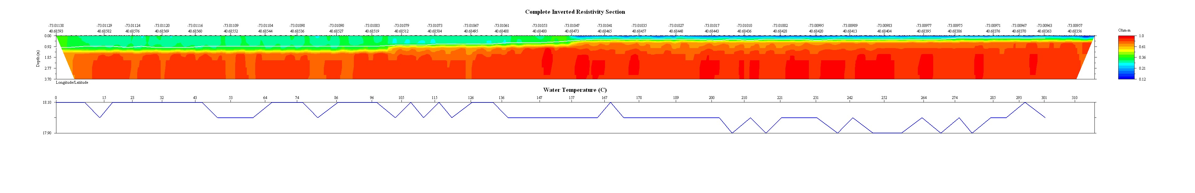
Sept. 24, 2008: Line L57F1, WRES = 0.29
EarthImager thumbnail JPEG image of line 57 resistivity and temperature profile.
MATLAB thumbnail JPEG image of line 57 resistivity profile.
Sept. 24, 2008: Line L58F1, WRES = 0.29
EarthImager thumbnail JPEG image of line 58 resistivity and temperature profile.
MATLAB thumbnail JPEG image of line 58 resistivity profile.
Sept. 24, 2008: Line L59F1, WRES = 0.29
EarthImager thumbnail JPEG image of line 59 resistivity and temperature profile.
MATLAB thumbnail JPEG image of line 59 resistivity profile.
Sept. 24, 2008: Line L60F1, WRES = 0.29
EarthImager thumbnail JPEG image of line 60 resistivity and temperature profile.
MATLAB thumbnail JPEG image of line 60 resistivity profile.
Sept. 24, 2008: Line L61F1, WRES = 0.29
EarthImager thumbnail JPEG image of line 61 resistivity and temperature profile.
MATLAB thumbnail JPEG image of line 61 resistivity profile.
Sept. 24, 2008: Line L62F1, WRES = 0.29
EarthImager thumbnail JPEG image of line 62 resistivity and temperature profile.
MATLAB thumbnail JPEG image of line 62 resistivity profile.
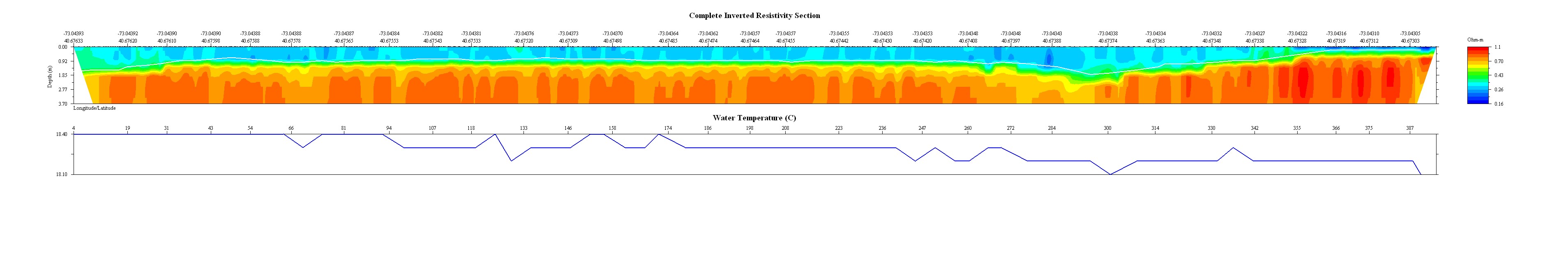
Sept. 24, 2008: Line L63F1, WRES = 0.29
EarthImager thumbnail JPEG image of line 63 resistivity and temperature profile.
MATLAB thumbnail JPEG image of line 63 resistivity profile.
Sept. 24, 2008: Line L64F1, WRES = 0.29
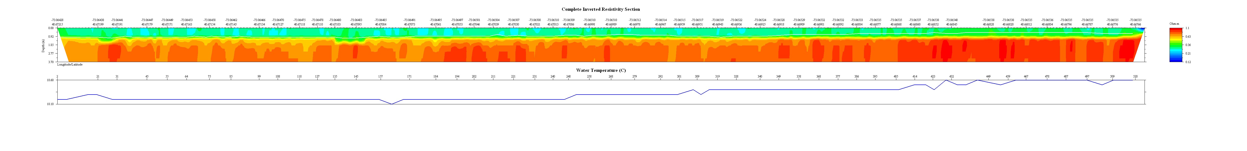
EarthImager thumbnail JPEG image of line 64 resistivity and temperature profile.
MATLAB thumbnail JPEG image of line 64 resistivity profile.

Accessibility FOIA Privacy Policies and Notices

Take Pride in America logo USA.gov logo U.S. Department of the Interior | U.S. Geological Survey
URL: http://pubsdata.usgs.gov/pubs/of/2011/1040/html/resistprev_sept15mb.html
Page Contact Information: GS Pubs Web Contact
Page Last Modified: Thursday, 08-Dec-2016 00:30:32 EST

Link to line 64 EarthImager and MATLAB JPEG profiles. Link to line 63 EarthImager and MATLAB JPEG profiles. Link to line 62 EarthImager and MATLAB JPEG profiles. Link to line 61 EarthImager and MATLAB JPEG profiles. Link to line 60 EarthImager and MATLAB JPEG profiles. Link to line 59 EarthImager and MATLAB JPEG profiles. Link to line 58 EarthImager and MATLAB JPEG profiles. Link to line 57 EarthImager and MATLAB JPEG profiles. Link to line 56 EarthImager and MATLAB JPEG profiles. Link to line 55 EarthImager and MATLAB JPEG profiles. Link to line 54 EarthImager and MATLAB JPEG profiles. Link to line 53 EarthImager and MATLAB JPEG profiles. Link to line 52 EarthImager and MATLAB JPEG profiles. Link to line 51 EarthImager and MATLAB JPEG profiles. Link to line 50 EarthImager and MATLAB JPEG profiles. Link to line 49 EarthImager and MATLAB JPEG profiles. Link to line 48 EarthImager and MATLAB JPEG profiles. Link to line 47 EarthImager and MATLAB JPEG profiles. Link to line 46 EarthImager and MATLAB JPEG profiles.