Click on figure for larger image.

Figure 8. Photograph of the autonomous surface vessel IRIS.

Figure 9. Map showing the comparison between the sea-floor surface generated from (A) gridding swath bathymetry data at the spacing of the seismic shot-point navigation supplemented with interpreted seismic-reflection profiles where swath data were unavailable and (B) the surface generated from all the high-resolution swath bathymetry data (available from Twichell and others, 2007).

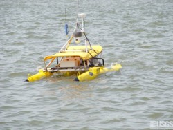
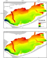
During 2005 and 2006 the USGS collected seismic-reflection data in Apalachicola Bay and St. George Sound off the coast of Florida. Data collected in 2005 were collected aboard the R/V Rafael, while in 2006 data were collected using the autonomous surface vessel IRIS (fig. 8) in addition to the R/V Rafael. In 2006 both platforms collected seismic data using an EdgeTech FSSB-424 system. The data aboard the R/V Rafael were recorded in SEG-Y format using SBLogger acquisition software, while the IRIS data were recorded in JSF format using EdgeTech JStar acquisition software. The seismic navigation and seismic-reflection profiles collected aboard the R/V Rafael are available from Twichell and others (2007).

While loading the seismic data into the seismic interpretation software, problems were discovered with the IRIS navigation released in Twichell and others (2007). Some of the seismic tracklines were missing, while other tracklines erroneously overlapped, resulting in duplicating sections of data. The Apalachicola Bay survey in 2006 was the first field deployment of the USGS IRIS system, and several data acquisition and processing issues had to be addressed. Acquisition settings, both hardware and software, were modified several times during the initial stages of the cruise until standardized settings could be established. The acquisition complications led to complications in the original processing of the data. By going back to the original JSF files collected during the survey, the missing tracklines were recovered and duplicate tracklines were eliminated. The corrected seismic-reflection profiles and navigation are available on the Data Catalog page of this report.

The reprocessed IRIS seismic-reflection data and navigation were loaded into Landmark SeisWorks software for interpretation along with the R/V Rafael data. The original R/V Rafael seismic data were acquired at two different sample rates: 40 microseconds (µs) and 80 µs. The IRIS seismic lines were also acquired at two sample rates: 23 µs and 46 µs. All data were resampled to 40 µs with PostStack data loader. Horizons were interpreted within the Landmark software, and these interpretations were exported as tab-delimited text files. Each exported text file contains four columns of information: line name, easting, northing, and milliseconds. The milliseconds column represents a two-way travel time. Each horizon was handled slightly differently when creating the geologic surfaces and these methods are discussed below. Since the primary purpose of collecting these data was to look at the Holocene evolution of Apalachicola Bay prior to human influences, anthropogenic modifications like channel dredging and spoil placement were excluded from the geologic surfaces created from the seismic interpretations.

The seismic data were processed utilizing numerous software packages. General processing of the IRIS seismic data used SIOSEIS (http://sioseis.ucsd.edu/), while Seismic Un*x (http://www.cwp.mines.edu/cwpcodes/) was used to produce JPEG images of each of the profiles. All seismic interpretation was done in Landmark SeisWorks software. ArcGIS 9.2 with Spatial Analyst was used to process the exported point data and generate the 75-m cell size grids of the interpreted horizons. For a more complete description of the processing steps used to generate the point datasets and the grids, see the metadata available on the Data Catalog page.

Sea Floor:

Swath bathymetry data were collected in Apalachicola Bay and published in Twichell and others (2007). This surface was also interpreted from the seismic-reflection data for two reasons: (1) gaps in the bathymetry data were covered by the shallow-water IRIS acquisition system and (2) interpolation over the shot-point navigation spacing allows validation of the interpolation techniques applied to the other interpreted horizons (fig. 9). The depths (in milliseconds) exported from Landmark represent the two-way travel times from the transducer to the sea floor and back. The depth of the transducer below the water surface was not accounted for, and tidal corrections were not performed. The tidal range in the study area is less than 0.5 m, which is within the accuracy of the data. Comparison of the seismic-reflection depths with the collocated high-resolution bathymetry allowed the derivation of a speed of sound in seawater. An accurate speed of sound estimate was needed for the conversion of travel time to depth. In determining the speed of sound value to be used, focus was placed on using data points with swath data in proximity to the locations that only had travel times. Although sound velocity measurements were taken during swath bathymetry data acquisition, those velocities consistently yielded depths too shallow for depths derived from the seismic data. A value of 1,700 meters per second (m/s) was used as the speed of sound in water for the R/V Rafael-collected seismic data where no swath data were available (depths greater than 2 m). In the extremely shallow areas (less than 2 m) where data were collected by the IRIS system, a similar method indicated an appropriate value for the speed of sound in water was 1,476 m/s. The higher value associated with the R/V Rafael data accounts for the seismic transducer depth that was not accounted for during acquisition and processing. Additionally, this value is in good agreement with the measured swath bathymetry depths in proximity to the shot points.

In order to generate the most accurate sea-floor surface possible, the shot-point navigation was used to extract bathymetry values from the 2-m resolution bathymetry data published in Twichell and others (2007). These data were supplemented with the sea-floor horizon interpreted from the seismic data where no swath bathymetry data were collected. Additionally, since these data are to be used to look at the Holocene evolution of Apalachicola Bay, points falling within 75 m of recent manmade features, such as the dredged Intracoastal Waterway and dredge spoil areas, were excluded from the interpolation process. The Apalachicola base map data published in Twichell and others (2007) were used to delineate the manmade features. ArcGIS 9.2 Spatial Analyst interpolation tool Topo to Raster was used to generate the surface from the seismic shot data with a cell size of 75 m.

Base of Mud:

These data are available as both a depth to the base of the modern mud surface and an isopach grid, both with a 75-meter cell size. This horizon presented the greatest challenge to represent in grid format due to the nature of the surface. The surface is narrowly separated from the sea floor, discontinuous, and often difficult to interpret on the seismic profiles. By making this an isopach grid, the absence of the horizon (zero thickness values) is distinguishable from the uninterpretable sections (no data), allowing the software to interpolate and create an isopach grid of appropriate extent. The milliseconds field in the point dataset represents two-way travel times of sediment thickness below the sea floor. A speed of sound in sediment of 1800 meters per second was used to convert the travel times to thicknesses. Points falling within 75 meters of manmade features were excluded from the interpolation process. Once the isopach grid was created, a depth surface was created by subtracting the isopach grid from the sea-floor grid.

Flooding Surface:

Within Landmark SeisWorks, the interpreted flooding surface was subtracted from the sea-floor horizon to yield an isopach horizon. The milliseconds field exported from Landmark represented the two-way travel time of the stratigraphic unit instead of the depth to the horizon. Although this surface exists throughout the study area, it is not always visible in the seismic profiles. The discontinuous nature of this horizon subsequently required the most extensive interpolation of all the grids. A speed of sound in sediment of 1,800 m/s was used to convert the two-way travel times to thicknesses, and interpolation of these values resulted in the isopach grid. This isopach grid was subtracted from the sea-floor surface to generate the flooding surface as a depth surface (75-m cell size). Only the depth surface is available on the Data Catalog page. As with the other surfaces, points falling within 75 m of manmade features were excluded from the interpolation process.

Lowstand Surface:

The lowstand surface was interpreted in Landmark SeisWorks. This horizon does not exist throughout the study area. In some areas where it is known to exist, its presence is obscured in the seismic profiles by gas in the overlying sediment or is absent due to insufficient depth penetration of the chirp system. The tab-delimited text file containing the line name, easting, northing, and milliseconds fields was exported from Landmark. The milliseconds field represents the two-way travel time from the water surface to the interpreted lowstand horizon.

In order to determine the true depth of the lowstand surface, the difference in the speed of sound in seawater and sediment needed to be accounted for. In order to accomplish this, the lowstand travel-time data points were joined with the sea-floor travel-time data points using a spatial join. After subtracting the sea-floor travel-time values from the lowstand travel-time values, one speed of sound in seawater and another travel time in sediment could be accounted for, resulting in a depth to surface in meters. The assumed speed of sound in the sediment is 1,800 m/s. These depth points were then interpolated following hydrologic rules as available in ArcGIS Spatial Analyst Topo to Raster tools. Although the horizon was not visible on all the seismic profiles, a generalized outline of the lowstand surface extent, combined with an assumed thalweg and the interpreted data points, was used to generate a 75-m cell size erosion surface that follows drainage rules. As with the sea-floor surface, points falling within 75 m of manmade features were excluded from the interpolation process.