Click on figures for larger images

Figure 4. Port-side view of the National Oceanic and Atmospheric Administration ship Thomas Jefferson at sea.

Figure 5. The National Oceanic and Atmospheric Administration (NOAA) launch 3102 being deployed from the NOAA ship Thomas Jefferson.

Figure 6. Starboard-side view of the National Oceanic and Atmospheric Administration launch 3102 at sea.

Figure 7. The RESON SeaBat 8125 multibeam echosounder hull-mounted to the National Oceanic and Atmospheric Administration launch 3101.

Figure 8. The RESON 7125 multibeam echosounder hull-mounted to the National Oceanic and Atmospheric Administration ship Thomas Jefferson.

Figure 9. Brooke Ocean Technology moving vessel profiler with a Sea-Bird Electronics, Inc. conductivity-temperature-depth profiler used to correct sound velocities for the multibeam data collected aboard the National Oceanic and Atmospheric Administration ship Thomas Jefferson.

Figure 10. Sea-Bird Electronics, Inc. SEACAT conductivity-temperature-depth profiler.

Figure 11. Comparison of the original reconnaissance multibeam bathymetry and the interpolated and regridded bathymetry for National Oceanic and Atmospheric Administration survey H12013.

Figure 12. Detailed planar view comparing the original reconnaissance multibeam bathymetry and the interpolated and regridded bathymetry from National Oceanic and Atmospheric Administration survey H12013.

Figure 13. A Klein 5000 sidescan-sonar system hull-mounted to a National Oceanic and Atmospheric Administration launch.

Figure 14. A port-side view of the U.S. Geological Survey Research Vessel Rafael, which was used to collect bottom photography and sediment samples for this study.

Figure 15. Locations of stations at which bottom samples and photographs were taken during cruise 09059 of Research Vessel Rafael to verify bathymetric and backscatter data.

Figure 16. The small Seabed Observation and Sampling System, a modified van Veen grab sampler equipped with still and video photographic systems, mounted on the aft starboard side of the U.S. Geological Survey Research Vessel Rafael.

Figure 17. Correlation chart showing the relationships among phi sizes, millimeter diameters, size classifications, and American Society for Testing and Materials and Tyler sieve sizes.

Figure 18. Sediment-classification scheme from Shepard, as modified by Schlee and Poppe and others.

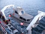
Multibeam Bathymetry

The NOAA ship Thomas Jefferson (fig. 4) and two 8.5-m aluminum Jensen launches (launch 3101 and launch 3102; figs. 5 and 6) deployed from the ship acquired multibeam bathymetric data from the study area over an approximately 29.1-km² area during 2009. The multibeam echosounder (MBES) data were collected with a hull-mounted RESON SeaBat 455-kilohertz (kHz) 8125 shallow-water system aboard launch 3101 (fig. 7) and RESON single frequency (400-kHz) 7125 systems aboard launch 3102 and the Thomas Jefferson (fig. 8). Horizontal positioning was by differential global positioning systems (DGPSs); HYPACK 2009 software was used for acquisition-line navigation. Sound-velocity corrections were derived with frequent conductivity-temperature-depth (CTD) profiles. A Brooke Ocean Technology moving vessel profiler (MVP) with an Applied Microsystems smart sound velocity and pressure (SV&P) sensor was used to collect sound and speed profile data from the ship (fig. 9). Manually deployed Sea-Bird Electronics, Inc. SBE-19+ CTD units were used to collect sound-speed profile data from the launches (fig. 10). Tidal-zone corrections were calculated from data acquired by the National Water Level Observation Network stations at New London (8461490) and New Haven (8465705), Conn. The vertical datum is mean lower low water. Detailed descriptions of the MBES acquisition and processing can be found in the Descriptive Report (National Oceanic and Atmospheric Administration, 2009a) and in the Data Acquisition and Processing Report (National Oceanic and Atmospheric Administration, 2009b).

The original vertical resolution of the multibeam bathymetric data was 0.5 m for water depths less than 20 m and 1 m for the deeper parts of the survey area. The bathymetric datasets were acquired and digitally logged with the HYSWEEP package of the HYPACK software and then processed by NOAA using the CARIS HIPS hydrographic image processing system software for quality control; this process incorporated sound velocity and tidal corrections and combined the datasets and HIPS imagery into a 2-m grid to produce the DTM. GeoTIFFs and grids were created with CARIS, Fledermaus, and ArcGIS software. The GeoTIFF imagery is vertically exaggerated fivefold and hill-shaded (sun-illuminated) from the northeast at an angle of 45 degrees (°) above the horizon. The original processed bathymetric dataset did not entirely cover the sea floor because line spacing during acquisition left areas of no data in many places between the ship's tracks (figs. 11 and 12). Therefore, the original data were interpolated and gridded to 10 m and combined with the 2-m grid. This process preserved the 2-m resolution in areas where multibeam coverage was complete but filled in the data gaps with the interpolated data. The bathymetric data are provided in the original reconnaissance and interpolated formats. A more detailed description of the acquisition parameters and processing steps performed by NOAA and the USGS to create the datasets presented in this report is included in the metadata files in the Data Catalog section of this report.

Sidescan Sonar

The sidescan-sonar data were acquired with a Klein 5000 sidescan-sonar system hull mounted to launch 3102 (fig. 13). The system was set to sweep 100 m to either side of the launch tracks. The system transmits at 455 kilohertzs (kHz). Daily confidence checks of the sidescan-sonar system were made by observing the outer ranges of the sonar images. Klein SonarPro was used to acquire the Klein 5000 sidescan-sonar data; the CARIS SIPS sidescan image processing system software was used to process the sidescan data and to produce a composite sidescan-sonar GeoTIFF image at 1-m horizontal resolution. Adobe Photoshop CS2 was used to apply a linear stretch (for instance, increase the dynamic range of the data), to change image from red-green-blue (RGB) color mode to 8-bit grayscale mode, to invert the grayscale image to make strong reflections light tones and weaker reflections darker tones, and to assign a 'NO DATA' value (255). ArcGIS 9.2 was used to project the image into Universal Transverse Mercator (UTM) Zone 18.

Sampling and Photography

Sediment sampling and bottom photography were conducted aboard the USGS Research Vessel (R/V) Rafael (fig. 14) during cruises 2009-059-FA in November 2009 and 2010-010-FA in April 2010. Surficial-sediment samples (0-2 cm below the sediment-water interface) and bottom photography were collected at 18 stations (fig. 15) with a modified van Veen grab sampler equipped with still- and video-camera systems (fig. 16). The photographic data were used to appraise intrastation bottom variability, faunal communities, and sedimentary structures (indicative of geological and biological processes) and to observe boulder fields where samples could not be collected. A gallery of images collected as part of this project is provided in the Bottom Photography section of this report; locations of the bottom photographs can be accessed through the Data Catalog section.

In the laboratory, the sediment samples were disaggregated and wet sieved to separate the coarse and fine fractions. The fine fraction (less than 62 micrometers) was analyzed by Coulter Counter, the coarse fraction was analyzed by sieving, and the data were corrected for salt content. Sediment descriptions are based on the nomenclature proposed by Wentworth (1922; fig. 17) and the size classifications proposed by Shepard (1954; fig. 18). A detailed discussion of the laboratory methods employed is given in Poppe and others (2005). Because biogenic carbonate shells commonly form in situ, they usually are not considered to be sedimentologically representative of the depositional environment. Therefore, gravel-sized bivalve shells and other biogenic carbonate debris were ignored. The grain-size analysis data can be accessed through the Data Catalog section of this report; a data dictionary is available in the Sediment Distribution section.

To facilitate interpretations of the distributions of surficial sediment and sedimentary environments, these data were supplemented by sediment data from compilations of earlier studies (Poppe and others, 1998a, 2000) and unpublished datasets from the NOAA National Geophysical Data Center. The interpretations of sea-floor features, surficial-sediment distributions, and sedimentary environments presented herein are based on data from the sediment-sampling and bottom-photography stations, on tonal changes in backscatter on the imagery, and on the bathymetry. For the purposes of this report, bedforms are defined by morphology and amplitude—sand waves (that is, subaqueous dunes) are higher than 1 m; megaripples are 0.2 to 1 m high; ripples are less than 0.2 m high (Ashley, 1990). The bathymetric grids and imagery released in this report should not be used for navigation.

To view files in PDF format, download a free copy of Adobe Reader.