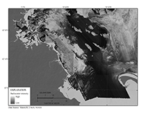
The following section describes how the geologic interpretations presented in this report were generated. Detailed descriptions of software, source information, scale, and accuracy assessments for each dataset are provided in the metadata files for geospatial data layers in the appendix.

Geophysical Data and Interpretations

During the past two decades, several organizations have collected acoustic backscatter, topography and bathymetry, and chirp seismic-reflection profile data within the coastal waters of Massachusetts (table 1). A seamless acoustic backscatter image and digital elevation model (DEM) were created from previously processed and published datasets (figs. 2 and 3; table 1). Each source backscatter mosaic GeoTIFF image was resampled to 10 meters per pixel (to achieve a common resolution) and mosaicked together (fig. 2) using PCI Geomatics (version 10.1). Each topographic and bathymetric source dataset was imported into ArcGIS (version 9.3.1), where all grids were resampled to 30 meters per pixel. The data were projected to a common horizontal coordinate system, and VDATUM (version 3.1; using the Maine, New Hampshire, Massachusetts-Gulf of Maine, version 01 (1983–2001) regional transformation grid) was used to define a common vertical coordinate system (North American Vertical Datum of 1988 (NAVD 88)). The grids were then mosaicked into a DEM using a blend algorithm (fig. 3).

More than 5,000 kilometers of chirp seismic-reflection profiles were collected and processed (table 1; fig. 4) using the techniques described in Barnhardt and others (2010) and Andrews and others (2010). Shallow stratigraphy and surficial geology interpretations were made in Landmark SeisWorks 2D (Haliburton, 2012) and consisted of (1) identifying and digitizing erosional unconformites defining the boundaries between Holocene, Pleistocene, and pre-Quaternary seismic units (figs. 5, 6, and 7); and (2) digitizing the extent over which each of the defined subsurface seismic units crops out on the seafloor (figs. 7 and 8).

Isochrons of the Holocene seismic units were exported and converted to thickness in meters using a constant seismic velocity of 1,500 meters per second (m/s). The resulting isopachs were imported into ArcGIS (version 9.3.1), as point features (easting, northing, and depth) and used to generate interpolated DEMs with 50-m cell sizes. The Holocene isopach DEMs were each added to a regional swath-bathymetry DEM (30-m cell size) to produce DEMs of the bounding unconformities (50-m cell sizes) relative to NAVD 88.

The digitized seafloor outcrops for each seismic unit were imported into ArcGIS as point features (easting, northing, seismic unit) and used to guide manual digitizing of polygons representing discrete areas of seismic-unit outcrop. The resulting polygon dataset provides a seamless representation of surficial geology for the seismic-reflection survey area (fig. 8).

Table 1: Data sources for the digital elevation model, backscatter mosaic, and seismic-reflection profile interpretations for the Inner Continental Shelf from Nahant to northern Cape Cod Bay, Massachusetts.s.

*These data were not used in the composite backscatter image.

Sediment Samples and Sediment Texture Classification Schemes

Sediment sample databases of Ford and Voss (2010) and McMullen and others (2011) were supplemented with National Oceanic and Atmospheric Administration chart sampling data and more than 2,000 bottom photographs and descriptions at more than 400 stations (fig. 9; Emily Huntley, CZM, unpub. data, 2012). This study used the Barnhardt and others (1998) and Shepard (1954), as modified by Schlee (1973), sediment texture classification schemes (figs. 10 and 11). The Barnhardt and others (1998) system is based on four basic, easily recognized sediment units: gravel (G), mud (M), rock (R), and sand (S). Because the sea floor is often a nonuniform mixture of these units, which are too small to define separately, the classification is further divided into 12 composite units, which are 2-part combinations of the 4 basic units (fig. 10). The classification is defined such that the primary unit, representing more than 50 percent of an area's texture, is given an upper case letter, and the secondary texture, representing less than 50 percent of an area's texture, is given a lower case letter. If one of the basic sediment units represents more than 90 percent of the texture, only its upper case letter is used. The units defined under the Barnhardt and others (1998) classification within this study area include Rg, Rs, Rm, Gr, Gs, S, Sg, Sm, M, and Ms. The Shepard (1954), as modified by Schlee (1973) (fig. 11), scheme for this study area includes gravel, sand, sandy-silt, silty-sand, and clay classes, with the addition of a solid class to encompass rocky areas.

Sediment Texture Mapping

The texture and spatial distribution of sea-floor sediment were analyzed qualitatively in ArcGIS using several input data sources, including acoustic backscatter, bathymetry, lidar, seismic-reflection profile interpretations, bottom photographs, and sediment samples (fig. 12). First, sediment texture polygons were outlined using backscatter intensity data (available at 1- to 10-m resolutions; table 1) to define changes in the seafloor based on acoustic return (fig. 2). Areas of high backscatter (light colors) have strong acoustic reflections and suggest boulders, gravels, and generally coarse seafloor sediments characterize the seafloor. Low-backscatter areas (dark colors) have weak acoustic reflections and generally are characterized by fine-grained material such as muds and fine sands.

The polygons were then refined and edited using gradient, rugosity, and hillshaded relief images derived from interferometric and multibeam swath bathymetry and lidar (available at 2.5- to 30-m resolutions; fig. 3; table 1). Areas of rough topography and high rugosity typically are associated with rocky areas, whereas smooth, low-rugosity regions tend to be blanketed by fine-grained sediment. These bathymetric derivatives helped to refine polygon boundaries where changes from primarily rock to primarily gravel may not have been apparent in backscatter data, but could easily be identified in hillshaded relief (fig. 12).

The third data input was the stratigraphic interpretation of seismic-reflection profiles, which further constrained the extent and general shape of seafloor sediment distributions and rocky outcrops, and also provided insight concerning the likely sediment texture based on the pre-Quaternary, glacial, or postglacial origin (figs. 8 and 12).

 Finally, bottom photographs and sediment samples (fig. 9) were used to define sediment texture for each polygon that was drawn using geophysical data (fig. 12). Average gravel, sand, silt, clay, and phi size for each sediment texture polygon were calculated using grain size statistics of sediment samples with laboratory analysis. Of the more than 5,000 samples total within the study area, 615 were analyzed in the laboratory for grain size. Samples with laboratory grain size analysis were preferred over visual descriptions when defining sediment texture throughout the study area. Sediment texture statistics can be found within the geospatial data file for sediment texture in the appendix. Average phi size and average particle content by weight data should be used cautiously in rock and gravel areas, where large particle sizes often are underrepresented using sediment sampling techniques. The average texture statistics in combination with the sediment sample count per polygon (where higher count numbers indicate a higher number of samples used in the average) are most applicable to the sand and silt sediment classes.

Some polygons had more than one sample, and some polygons lacked sample information. For multiple samples within a polygon, the dominant sediment texture (or average phi size) was used to classify sediment type. In rocky areas, bottom photographs were used in the absence of sediment samples to qualitatively define sediment texture. Polygons that lacked sample information were defined texturally through extrapolation from adjacent or proximal polygons of similar acoustic character that did contain sediment samples.

Physiographic Zones

The distribution of seafloor physiographic zones was analyzed qualitatively in ArcGIS using the same input sources and digitization techniques used to determine sediment texture and distribution. Following the methods used in the Gulf of Maine to produce geologic maps (Kelley and Belknap, 199; Kelley and others, 1996; Barnhardt and others, 2006; and Barnhardt and others, 2009), the seafloor within the study area was divided into physiographic zones based on seafloor morphology and dominant sediment texture. Physiographic mapping allows efficient mapping of large areas and presents geomorphic and textural data in a single classification scheme. This simplified designation especially is useful in complex inner-shelf settings such as northeastern Massachusetts, New Hampshire, and Maine. An added advantage of physiographic zones is that they do not require full data coverage and can be defined from a variety of data sources. Physiographic zones identified within the study area include rocky zones, outer basins, nearshore basins, ebb-tidal deltas, hard-bottom plains, nearshore ramps, sand waves, shelf valleys, and dredged channels. These zones are further described in the “Results” section in terms of their location, size, morphology, geologic setting, and substrate properties.

Figure 2. A composite backscatter image at 10-meter resolution was created from a series of published backscatter images (table 1). Areas of high backscatter have strong acoustic reflections and suggest boulders, gravels, and generally coarse seafloor sediments. Low backscatter areas have weak acoustic reflections and are generally finer grained material such as muds and fine sands.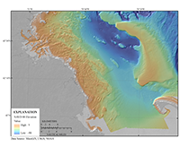

Figure 3. A digital elevation model (DEM) was produced from swath interferometric, multibeam bathymetry, and lidar at 30-meter resolution (table 1). High rugosity and high relief are most often associated with rocky areas, whereas smooth, low relief regions tend to be blanketed by fine-grained sediment deposits.  NAVD 88, North American Vertical Datum of 1988.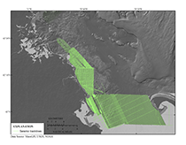

Figure 4. Map showing tracklines of chirp seismic-reflection profiles from Andrews and others (2010) and Barnhardt and others (2010) used to interpret surficial geology and shallow stratigraphy.

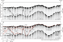
Figure 5.Chirp seismic reflection profiles A, A-A’ with seismic stratigraphic interpretation and B, illustrating the subsurface stratigraphy of the study area. Qmn, Holocene nearshore marine sediments; Qfe, Holocene fluvial and estuarine sediments; Qd, undifferentiated Pleistocene glacial drift sediments; Pz(?)/Tcp(?)/Qt(?), undifferentiated Paleozoic bedrock, late-Cretaceous to Tertiary coastal plain sediments, or Pleistocene glacial tills; Ul, fluvial unconformity marking the upper surface of Pz(?)/Tcp(?)/Qt(?); Ur, late Wisconsinan regressive unconformity; Ut, transgressive unconformity over Qfe and Qd. See figure 6 for detailed descriptions of stratigraphic units and major unconformities (indicated by red lines). See figure 8 for profile location. A constant sound velocity of 1,500 meters per second was used to convert two-way travel time to depth in meters.

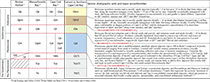
Figure 6.  Seismic stratigraphic units and major unconformities interpreted within Boston Harbor by Rendigs and Oldale (1990), Massachusetts Bay by Oldale and Bick (1987), Cape Cod Bay by Oldale and O’Hara (1990), and between Nahant and northern Cape Cod Bay in this study.

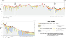
Figure 7. Geologic cross sections (B–B′ and C–C′) illustrating the general distributions and thicknesses of seismic stratigraphic units and elevations of major unconformities beneath the Massachusetts inner shelf between Nahant and northern Cape Cod Bay. Geologic cross sections are interpreted from chirp seismic reflection profiles. Vertical scale is elevation in meters from the North American Vertical Datum of 1988. Solid vertical black line denotes bend in section, and dashed vertical black lines indicate intersections. See figure 6 for descriptions of stratigraphic units and unconformities. Geologic section locations are identified on figure 8.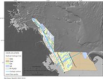

Figure 8.Surficial geologic map of the Massachusetts inner shelf between Nahant and northern Cape Cod Bay. The areal extents over which subsurface geologic units crop out at the seafloor were interpreted from seismic-reflection data. Detailed descriptions of the primary geologic units are figure 6. Qmn, Holocene nearshore marine sediments; Qmd, Holocene deepwater marine sediments; Qfe, Holocene fluvial and estuarine sediments; Qd, undifferentiated Pleistocene glacial drift sediments; Pz(?)/Tcp(?)/Qt(?), undifferentiated Paleozoic bedrock, late Cretaceous to Tertiary coastal plain sediments, or Pleistocene glacial tills. Holocene sediment veneers too thin to be detected in the seismic-reflection data (less than about 0.5 meter) may overlie outcrops of pre-Holocene units (blue and gray areas) locally. The locations of geologic cross sections B-B' and C-C' (fig. 8) are indicated by cyan lines, and the locations of chirp seismic-reflection profiles A-A', D-D', E-E', and F-F' are indicated by black lines.

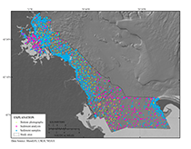
Figure 9. Bottom photographs and sediment samples collected within the study area were used to aid interpretations. Sediment samples with laboratory analysis are shown as magenta dots, while blue dots are visual descriptions. Data are from Ford and Voss (2010), McMullen and others (2011) and Emily Huntley (Massachusetts Office of Coastal Zone Management, unpub. data, 2012).

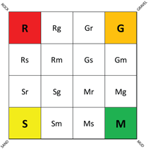
Figure 10. Barnhardt and others (1998) bottom-type classification based on four basic sediment units: rock (R), gravel (G), sand (S), and mud (M). Twelve additional two-part units represent combinations of the four basic units, where the primary texture (more than 50 percent of the area) is given an upper case letter and the secondary texture (less than 50 percent of the area) is given a lower case letter.

Figure 11.Sediment classification scheme by Shepard (1954), as modified by Schlee (1973) and McMullen and others (2011).

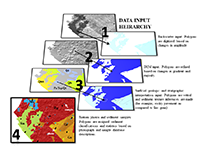
Figure 12. Sediment texture and distribution data were mapped qualitatively in Esri ArcGIS using a hierarchical methodology. Backscatter data were the first input, followed by bathymetry, surficial geologic and shallow stratigraphic interpretations, and photograph and sample databases. DEM, digital elevation model.