Open-File Report 2016-1119
Shallow Geology, Sea-Floor Texture, and Physiographic Zones of Vineyard and Western Nantucket Sounds, Massachusetts
MethodsThe following section describes how the geologic interpretations presented in this report were generated. Detailed descriptions of software, source information, scale, and accuracy assessments for each data set are provided in the metadata files for each data set in Appendix 1 — Geospatial Data. High-resolution bathymetry, acoustic-backscatter, and seismic-reflection data collected by the USGS, the National Oceanic and Atmospheric Administration (NOAA), and the U.S. Army Corps of Engineers (USACE) provide nearly full coverage of the sea floor in the 494 square kilometer (km2) study area (fig. 1, table 1). The new geophysical data, sediment samples, and sea-floor photographs/video allowed for interpretation of seafloor composition and shallow subsurface stratigraphy at finer scales and resolutions than previously possible. However, the interpretations do have limitations, which primarily arise from the types, quality, and density of data from which they were made. Pendleton and others (2013) provide detailed discussion regarding the limitations associated with these surficial mapping methods. Consequently, qualitative confidence levels were assigned to some interpretations and must be considered when surficial maps are used to guide management decisions and future research. Bathymetric and Backscatter CompositeBathymetric data previously published by the USGS, NOAA, and USACE (table 1) were utilized as source data to create a bathymetric digital elevation model (DEM) covering nearly the entire study area (fig. 3). The bathymetric DEM is referenced to the North American Vertical Datum of 1988 (NAVD 88). Source datasets originally referenced to tidal datums were converted to NAVD 88 by using VDATUM (version 3.2). Bathymetric source data were compiled in an ArcGIS (version 9.3.1) terrain dataset. In areas of overlap between source datasets, higher resolution and more recently collected data were generally retained, while lower resolution and older data were eliminated. Consequently, the final bathymetric DEM (fig. 3), gridded at a 10-m-per-pixel resolution, is composed of the highest quality bathymetric data available for Vineyard and western Nantucket Sounds at the time of this publication. Vertical resolutions of the source data range from unknown, for lead-line soundings, to 0.1 m, for interferometric, multibeam, and lidar swath bathymetric data. A seamless acoustic backscatter image was also created (fig. 4) from data previously published by USGS and NOAA (table 1). If necessary, source backscatter data published at resolutions finer than 1-m were resampled to a common 1-meter-per-pixel resolution. Finally, all source images were mosaicked into a composite GeoTIFF by using PCI Geomatica (version 10.1). Table 1. Sources of bathymetry, backscatter, and seismic-reflection data used in the Vineyard and western Nantucket Sounds, Massachusetts study area. [JALBTCX, Joint Airborne Lidar Bathymetry Technical Center of Expertise; lidar, light detection and ranging; kHz, kilohertz]
1Data collected by National Oceanic and Atmospheric Administration. 2Data collected by U.S. Army Corps of Engineers. 3Data collected by U.S. Geological Survey. Seismic Stratigraphic and Surficial Geologic MappingApproximately 4,500 kilometers of seismic-reflection profiles, collected between 2009 and 2011 (table 1, fig. 5), were interpreted in Landmark SeisWorks 2D (version R5000). Most of the profiles were collected by using chirp sonars with broadband frequencies of 4 to 24 and 0.5 to 12 kilohertz (kHz) or narrow-band frequencies centered around 3.5 kHz. Additional profiles were collected by using a boomer source and multichannel streamer (16 channels with a 3.125-m group interval) in select locations. Legacy seismic-reflection data (O’Hara and Oldale, 1980, 1987; McMullen and others, 2009) were used in the interpretations for general correlation with the seismic stratigraphy interpreted in previous studies. Interpretations of shallow stratigraphy and surficial geology were conducted in the time domain (two-way traveltime) and consisted of (1) identifying and defining seismic stratigraphic units on the basis of seismic facies, and digitizing reflectors (horizons) defining the boundaries between individual seismic stratigraphic units; and (2) digitizing the extent over which each of the defined seismic stratigraphic units crops out on the sea floor. Two-way traveltime values of the postglacial seismic units were exported and converted to thickness in meters by using a constant seismic velocity of 1,500 meters per second (m/s). The resulting isopach values were imported into ArcGIS as point features (easting, northing, thickness) and used to generate interpolated DEMs with 40-m-per-pixel resolutions. Each isopach DEM was added to the regional swath-bathymetry DEM (fig. 3) to produce DEMs of the bounding unconformities (40-m cell sizes) relative to NAVD 88. The digitized sea-floor outcrops for each seismic unit were imported into ArcGIS as point features (easting, northing, seismic unit) and used to guide manual digitizing of polygons representing discrete areas of seismic-unit outcrop. The resulting polygon dataset provides a seamless representation of surficial geology for the seismic-reflection survey area. The surficial geology polygons also provide insight into the likely sediment texture at the sea floor on the basis of the glacial or postglacial (mostly marine) origin and depositional environment inferred from the seismic interpretation. The geologic observations were incorporated into surficial sediment texture mapping. High-density, seismic-reflection data were collected only within the areas surveyed by the USGS between 2009 and 2011 (table 1, fig. 5). As a result, surficial geology polygons derived from the seismic interpretations are less extensive than the sea-floor sediment texture and physiographic zone polygons, which cover areas equivalent to the composite bathymetry (fig. 3). Sediment Samples and Sediment Texture Classification SchemeSediment samples from the databases of Ford and Voss (2010) and McMullen and others (2012) were supplemented with NOAA nautical chart sample information and visual descriptions of sea-floor photographs compiled by CZM (Emily Huntley, CZM, written communication, 2014). These resources contained laboratory analysis data for samples collected at 222 locations and visual observation data from 4,715 locations within the study area (fig. 6). Additional observations were made from 1,786 sea-floor photographs collected by the USGS (fig. 6; Poppe and others, 2007, 2008, 2010; Ackerman and others, 2015). We used the Barnhardt and others (1998) sediment texture classification scheme (fig. 7), which is effective for describing sea-floor texture on the New England inner continental shelf where reworked glacial drift and rocky pavements are common. The Barnhardt and others (1998) classification defines surficial sediment types primarily on the basis of acoustically assessed sea-floor characteristics, including reflectivity (sidescan-sonar backscatter) and bathymetric relief. The acoustic data reveal fine-scale areal variability in sea-floor character that would be largely undetected by grid-sampling methods. Barnhardt and others (1998) use geologic and geophysical data to correlate and support interpretation of the acoustically defined sea-floor units. Their classification scheme defines four basic, easily recognized sediment units: Rock (R), Gravel (G), Sand (S), and Mud (M). Because the sea floor is often a nonuniform mixture of these units, which are too small to define separately, the classification is further divided into twelve composite units, which are two-part combinations of the four basic units (fig. 7). The classification is defined such that the primary unit, representing more than 50 percent of an area's texture, is given an uppercase letter, and the secondary texture, representing less than 50 percent of an area's texture, is given a lowercase letter. If one of the basic sediment units represents more than 90 percent of the texture, only its uppercase letter is used. Sediment Texture MappingAreas of similar sea-floor sediment texture were defined through integrated analysis of acoustic-backscatter, bathymetry, seismic-reflection profile interpretations, sediment samples, and bottom photographs by using methods similar to those described by Pendleton and others (2013) and Foster and others (2015). Sediment texture polygons were digitized in ArcGIS at scales between 1:5,000 and 1:20,000, depending on the resolution of the source data, but the recommended scale for application of these data is greater than 1:25,000. Polygons were initially digitized on the basis of acoustic backscatter intensity and patterns (fig. 4). High-backscatter areas with strong acoustic reflectivity are indicative of boulders, gravels, and generally coarse sea-floor sediments, whereas low-backscatter areas with weak acoustic reflectivity typically indicate finer grained material such as sands and muds. Backscatter patterns are useful for identifying zones of homogeneous sea-floor environments, such as boulder fields, cobble pavements, sand sheets (with or without bedforms), or anthropogenic features, as well as the gradational or sharp boundaries between them. The polygons interpreted from backscatter data were then refined on the basis of sea-floor morphology interpreted from the bathymetry and depth derivatives, including gradient, rugosity, and hillshade relief. Areas of rough topography and high rugosity are associated with rocky areas or places where surficial sediments form sand waves and rippled bedforms, whereas smooth, low-relief regions tend to represent hard-bottom plains or areas blanketed by fine-grained sediments. In areas where backscatter data were not available, bathymetry and the bathymetric derivatives were used to create the initial polygons. Stratigraphic interpretations of seismic-reflection profiles were also used to refine the polygons; these interpretations provided additional constraints over areal extents of rocky and gravelly areas and insights concerning the likely sediment texture based on the glacial or postglacial origin of the seismic facies associated with surficial units. Finally, sediment texture data and bottom photographs were used to verify and refine the classification of the sediment texture polygons. Samples with laboratory analysis data, rather than qualitative descriptions, were preferred for defining sediment texture throughout the study area. Bottom photographs were also used to qualitatively define sediment texture, particularly in areas dominated by gravel- to boulder-size material. Many of the sediment type polygons did not contain sample information. For these polygons, sediment textures were extrapolated from proximal polygons that contained samples and produced similar acoustic backscatter and seismic-reflection properties. Table 2. Confidence levels assigned to sediment texture polygons on the basis of the data used in the interpretation. The spatial distribution of polygons and associated confidence levels are shown in figure 8. [lidar; light detection and ranging]
Sediment texture polygons were assigned one of five confidence levels on the basis of the type and quality of data used to define them (table 2). The confidence levels were attached as an attribute in the geographic information system (GIS) for each sediment texture polygon (fig. 8). Level-one confidence areas contain the widest variety of high-resolution geophysical data and the highest quality sediment sample data. Level-two areas share the same variety of geophysical data but did not contain sediment samples that were analyzed quantitatively in the laboratory. Many level-two areas consist of gravel or gravelly sediment from which there was no attempt to collect a physical sample, or sample attempts recovered no material. This lack of samples is a common problem because most bottom samplers are either incapable of sampling gravel and cobble or do so inaccurately. Because level-three areas were designated in the absence of seismic-reflection data and possibly sediment samples with laboratory analyses, these areas are considered to have slightly less confidence than level-one and level-two areas. Level-four and level-five areas have substantially lower confidence because the primary component of the Barnhardt and others (1998) classification, acoustic reflectivity, is lacking. Consequently, levels one through three are generally considered “high confidence,” and levels four and five are considered “low confidence” (table 2). Physiographic ZonesBased on geologic maps produced for the western Gulf of Maine (Kelley and Belknap, 1991; Kelley and others, 1998; Barnhardt and others, 2006, 2009), and Massachusetts, Cape Cod, and Buzzards Bays (Pendleton and others, 2013; Foster and others, 2015), the sea floor of Vineyard and western Nantucket Sounds was divided into physiographic zones, which are delineated on the basis of sea-floor morphology and dominant sediment texture. Physiographic mapping allows for efficient characterization of large areas by utilizing a variety of data sources that may not provide full sea-floor coverage. The zones were defined qualitatively in ArcGIS by using the same data sources and digitization techniques used to derive sediment texture and distribution. |

![]() U.S. Department of the Interior |
U.S. Geological Survey
U.S. Department of the Interior |
U.S. Geological Survey
URL: http://pubsdata.usgs.gov/pubs/of/2016/1119/ofr20161119_methods.html
Page Contact Information: GS Pubs Web Contact
Page Last Modified: Wednesday, 11-Oct-2017 17:56:39 EDT