 | List of Figures
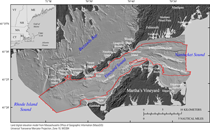 |
Figure 1. Location map of the Vineyard and western Nantucket Sounds study area, and inset map illustrating the study area location within southern New England. Swath bathymetry, acoustic backscatter, and chirp seismic-reflection data were collected in the area inside the red polygon. Dark gray is from a Massachusetts Office of Geographic Information (MassGIS) hillshade relief image of Massachusetts. Medium gray is from the hillshade relief maps derived from the composite bathymetry of Buzzards Bay (Foster and others, 2015) and Vineyard and western Nantucket Sounds (fig. 3). |
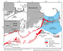 |
Figure 2. Map showing glacial moraines on land and submerged on the continental shelf (compiled from Stone and others, 2005; Boothroyd, 2008; Stone and DiGiacomo-Cohen, 2009; and Stone and others 2011), ice-front locations for southern New England (from Ridge, 2004), and glacial lakes and associated outlet spillways (compiled from Larsen, 1982; Uchupi and Mulligan, 2006). Inset illustrates the relative locations of four lobes of the Laurentide ice sheet in southeastern New England (modified from Oldale and Barlow, 1986). Figure is modified from Foster and others (2015). |
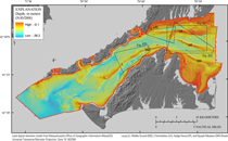 |
Figure 3. A digital elevation model (DEM) produced from swath (interferometric, multibeam, and lidar; collected within the red polygon) and single-beam (collected outside the red polygon) bathymetric data gridded at a 10-meter-per-pixel horizontal resolution (table 1). Black polygons indicate areas of figures 21 and 22. Depth is referenced to the North American Vertical Datum of 1988. The locations of Lucas (L), Middle Ground (MG), L'Hommedieu (LH), Hedge Fence (HF), and Squash Meadow (SM) Shoals are also indicated. |
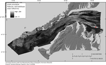 |
Figure 4. A composite backscatter image at 1-meter resolution, created from a series of published backscatter images (table 1). Areas of high backscatter (light gray tones) have strong acoustic reflections and suggest boulders, gravels, and generally coarse sea-floor sediments. Low-backscatter (dark gray to black tones) areas have weak acoustic reflections and generally indicate finer grained material such as fine sands and muds. Red star shows location of figure 20. |
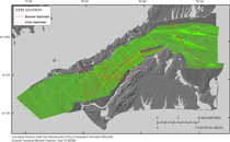 |
Figure 5. Map showing tracklines of chirp and boomer seismic-reflection profiles (table 1) used to interpret surficial geology and shallow stratigraphy. The bathymetric hillshade relief map is derived from the composite bathymetry shown in (fig. 3). |
 |
Figure 6. Map showing locations of observations of sea-floor composition used to aid the geophysical and geologic interpretations (Ford and Voss, 2010; McMullen and others, 2012; Emily Huntley, Massachusetts Office of Coastal Zone Management, written communication, 2014). Blue dots indicate visual descriptions made from sediment grab samples, vibracore tops, or sea-floor photographs/video, or visual descriptions obtained from National Oceanic and Atmospheric Administration nautical charts (generally near the shoreline). Magenta dots indicate sediment grab samples that were analyzed in a laboratory to obtain grain-size statistics. Processed samples are preferred over those that were only described visually. Bottom photograph locations, indicated by yellow dots, are generally associated with sites where samples were collected and grain-size statistics were processed. The bathymetric hillshade relief map is derived from the composite bathymetry shown in figure 3. |
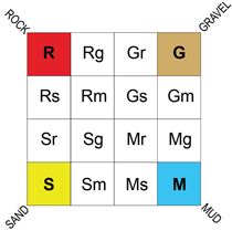 |
Figure 7. Barnhardt and others (1998) bottom-type classification based on four basic sediment units: Rock (R), Gravel (G), Sand (S), and Mud (M). Twelve additional two-part units represent combinations of the four basic units. In the two-part units, the primary texture (greater than 50 percent of the area) is given an uppercase letter and the secondary texture (less than 50 percent of the area) is given a lowercase letter. Only the uppercase letter is used for areas where more than 90 percent of the texture is represented by one basic sediment unit. Figure is modified from Barnhardt and others (1998). |
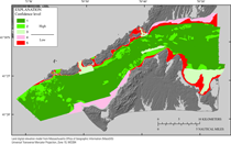 |
Figure 8. Map showing the distribution of confidence levels for sediment texture interpretation (table 2) within the Vineyard and western Nantucket Sounds study area. |
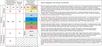 |
Figure 9. Seismic stratigraphic units and major unconformities interpreted within Vineyard Sound and eastern Rhode Island Sound by O'Hara and Oldale (1980), within Nantucket Sound by O'Hara and Oldale (1987), and by this study. m, meters. |
 |
Figure 10. Chirp seismic-reflection profile A-A' with seismic stratigraphic interpretation. This profile illustrates the stratigraphy beneath western Vineyard Sound, between Cuttyhunk Island and Aquinnah on Martha's Vineyard. See figure 9 for descriptions of stratigraphic units and major unconformities (indicated by red lines). Deformed Late Cretaceous(?) to early(?) Pleistocene coastal plain units (QTKu?) underlie ice-marginal till that forms an east-west extension of the Martha's Vineyard end moraine (Qdm) across western Vineyard Sound. The deep basin north of the morainal dam is mostly filled by thick glacial lacustrine (Qdl) units, which are unconformably overlain by less extensive glaciofluvial outwash (Qdf) and Holocene fluvial, estuarine (Qfe), and nearshore and deepwater marine (Qmn and Qmd, respectively) deposits. The morphologies of meltwater drainage incised across the outwash plain through the morainal dam are apparent. To the southwest, Buzzards Bay end moraine deposits extend across previously deposited glacial drift. See figures 14 and 17 for profile location. Dashed vertical black line indicates intersection with profile B-B’. A constant sound velocity of 1,500 meters per second was used to convert two-way traveltime to depth in meters. |
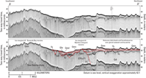 |
Figure 11. Chirp seismic-reflection profile B–B' with seismic stratigraphic interpretation. This profile illustrates the stratigraphy beneath western Vineyard Sound, between Cuttyhunk Island and Aquinnah on Martha’s Vineyard. See figure 9 for descriptions of stratigraphic units and major unconformities (indicated by red lines). Deformed Late Cretaceous(?) to early(?) Pleistocene coastal plain units (QTKu?) underlie ice-marginal till that forms an east-west extension of the Martha's Vineyard end moraine (Qdm) across western Vineyard Sound. The deep basin north of the morainal dam is mostly filled by thick glacial lacustrine (Qdl) units, which are unconformably overlain by less extensive glaciofluvial outwash (Qdf) and Holocene fluvial, estuarine (Qfe), and nearshore and deepwater marine (Qmn and Qmd, respectively) deposits. The morphologies of meltwater drainage incised across the outwash plain through the morainal dam are apparent. To the southwest, Buzzards Bay end moraine deposits extend across previously deposited glacial drift. See figures 14 and 17 for profile location. Dashed vertical black line indicates intersection with profile A-A’. A constant sound velocity of 1,500 meters per second was used to convert two-way traveltime to depth, in meters. |
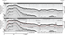 |
Figure 12. Chirp seismic-reflection profile C–C' with seismic stratigraphic interpretation. This profile illustrates the stratigraphy beneath northwestern Nantucket Sound in the vicinity of L'Hommedieu Shoal. See figure 9 for descriptions of stratigraphic units and major unconformities (indicated by red lines). Ice-contact material (Qdt) with a steep northern margin is covered by relatively thick, ice-proxal outwash (Qdf) that grades ice-distally and southward to terraced outwash plains (Qdf). Fluvial and estuarine fills (Qfe) are restricted to the topographic lows of outwash channels in the regressive unconformity Ur, and sandy Holocene sediments, reworked from the underlying drift, form relatively thick draping shoals and mobile sand waves (Qmn) across the ice-marginal core locally. See figures 14 and 21 for profile location. A constant sound velocity of 1,500 meters per second was used to convert two-way traveltime to depth, in meters. |
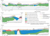 |
Figure 13. Geologic sections (D-D', E-E', and F-F') illustrating the general distributions and thicknesses of seismic stratigraphic units and major unconformities beneath Vineyard and western Nantucket Sounds. The geologic sections were produced from chirp and boomer seismic-reflection profile interpretations. See figure 9 for descriptions of stratigraphic units and unconformities. Geologic section locations are indicated on figure 14. |
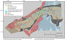 |
Figure 14. Map showing the surficial geology of Vineyard and western Nantucket Sounds with equivalent onshore geology (adapted from Stone and DiGiacomo-Cohen, 2009). The areal extents over which offshore subsurface geologic units crop out at the sea floor were interpreted from seismic-reflection data. See figure 9 for detailed descriptions of the offshore geologic units. Holocene sediment veneers too thin to be detected in the seismic data (less than approximately 0.5 m) may overlie outcrops of older units locally. The bathymetric hillshade relief map is derived from the composite bathymetry in figure 3. Black lines indicate chirp profile locations (figs. 10, 11, and 12) and red lines indicate geologic section locations (fig. 13). Qdm, Pleistocene glacial moraine – Martha's Vineyard and Buzzards Bay moraines; Qdt, undifferentiated Pleistocene glacial till and ice contact; Qdl, Pleistocene glaciolacustrine (glaciodeltaic and lake floor) Qdf, Pleistocene glaciofluvial (outwash); Qfe, Holocene fluvial and estuarine; Qmn and Qmd, Holocene nearshore and deepwater marine. The locations of Lucas (L), Middle Ground (MG), L’Hommedieu (LH), Hedge Fence (HF), and Squash Meadow (SM) Shoals are also indicated. |
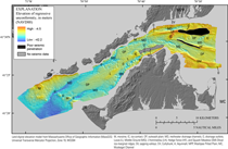 |
Figure 15. Map showing the elevation (referenced to the North American Vertical Datum of 1988) of the late Wisconsinan to early Holocene age regressive unconformity Ur, which identifies the eroded surface of Pleistocene glacial drift beneath Vineyard and western Nantucket Sounds. Ur represents a composite unconformity where it locally merges with the fluvial unconformity U1 at the base of Pleistocene sediments or is truncated by the Holocene transgressive unconformity (Ut). The surface illustrates the topographic morphologies of prominent glacial features in the shallow subsurface, including high-relief bouldery moraines (M) and ice-contact deposits (IC), moderate-relief ice-marginal drift ridge cores of Lucas (L), Middle Ground (MG), L'Hommedieu (LH), Hedge Fence (HF), and Squash Meadow (SM) shoals, fluvial drainage outlets cut through ice-marginal sills (O), relatively low-relief outwash plains (OP), and linear-to-sinuous depressions of meltwater drainage channels (MD). SV, sapping valleys; CH, Cuttyhunk; A, Aquinnah; MPP, Mashpee Pitted Plain; MC, Muskeget Channel. |
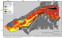 |
Figure 16. Map showing the thickness of postglacial fluvial and estuarine (Qfe) and Holocene nearshore and deepwater marine (Qmn and Qmd, respectively) sediments beneath Vineyard and western Nantucket Sounds. The bathymetric hillshade relief map is derived from the composite bathymetry in figure 3. The black polygon depicts the boundary of the seismic-survey area. The locations of Lucas (L), Middle Ground (MG), L’Hommedieu (LH), Hedge Fence (HF), and Squash Meadow (SM) Shoals are also indicated. |
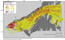 |
Figure 17. Map showing the distribution of sediment textures within Vineyard and western Nantucket Sounds on the basis of the bottom-type classification from Barnhardt and others (1998) (fig. 7). The green polygon is indicative of general confidence level of the interpretations, with high-confidence interpretations inside, and low-confidence interpretations outside. The black rectangle shows the extent of figure 18, and black lines show the locations of seismic profiles A-A' and B-B' from figures 10 and 11, respectively. The bathymetry hillshade relief map underlying the sediment texture layer is derived from the composite bathymetry in figure 3. |
 |
Figure 18. A, Map showing sediment textures within an approximately 6-square-kilometer area of western Vineyard Sound, between Aquinnah on Martha’s Vineyard and Cuttyhunk Island (see fig. 17 for location; see fig. 7 for bottom-type classification). The locations of seismic profiles A–A' (fig. 10) and B–B' (fig. 11) are indicated by black lines. The bathymetric hillshade relief map underlying the sediment texture layer is derived from the composite bathymetry in figure. 3. B, A photograph of sandy sediment obtained from a section of sea floor classified as primarily Sand (S). C, a photograph of the sea floor showing boulders within an area classified as primarily rock with gravel (Rg). D, A photograph from a section of sea floor classified as primarily sand with some mud (Sm). The scales of photographs B-D are approximately 60, 100, and 65 centimeters, respectively. |
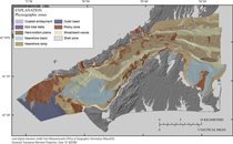 |
Figure 19. Map showing the distribution of physiographic zones within Vineyard and western Nantucket Sounds. The physiographic zone classification is adapted from Kelley and others (1998), and the zones are delineated on the basis of sea-floor morphology and the dominant texture of surficial material. The bathymetric hillshade relief map underlying the sediment texture layer is derived from the composite bathymetry in figure 3. |
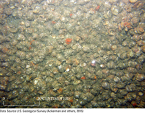 |
Figure 20. Bottom photograph showing a section of sea floor within Nantucket Sound composed of muddy sand covered by highly concentrated Crepidula fornicata (from Ackerman and others, 2015). The shells produce a continuous high-backscatter zone on the regional acoustic backscatter imagery, despite overlying a substrate primarily composed of muddy sand. See figures 4 and 19 for locations of the photograph and the shell zone from which it was obtained. |
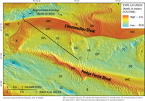 |
Figure 21. Detailed bathymetric map of Nantucket Sound in the vicinity of L’Hommedieu and Hedge Fence Shoals. The presence of large sand waves (SW) with fields of smaller rippled bedforms superimposed upon them clearly identify the extents of the sandy shoal deposits. Where the sandy sediments thin, deglacial morphologies, including the ice-marginal drift ridge cores (IMC) underlying the shoals, drainage outlets cut through the ice-marginal cores (O), outwash plains (OP; OPu, upper; Opl, lower), outwash channels (OC), ice-contact deposits possibly in the form of kame (K) and esker (E), and kettle holes (KH), are clearly identifiable across the adjacent sea floor. While the deglacial morphologies are well preserved between these shoals, they are significantly subdued within the main channel of the sound to the south of Hedge Fence Shoal, presumably due to differential erosion of the sea floor by wave and tidal currents during marine transgression. Barchanoid bedforms (B) are indicative of sediment transport in the presence of strong tidal currents within the main channel of the sound. Black arrows identify the inferred directions of drainage entering Nantucket Sound from the Mashpee Pitted Plain (fig. 1) as flow was divided upon intersecting L’Hommedieu Shoal. Black line indicates location of seismic reflection profile C - C’ (fig. 12). See figure 14 for map location. |
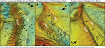 |
Figure 22. Three oblique bathymetric views of the sea floor surrounding A, Lucas and Middle Ground Shoals, B, L’Hommedieu Shoal, and C, Hedge Fence Shoal illustrating places where the sandy Holocene components (LMSS, laterally migrating sand shoal) of each shoal are oriented obliquely to the trends of their underlying ice-marginal drift ridge cores (IMC). While achieving dynamic equilibrium in the presence of opposing tidal currents, the shoals have in places migrated sufficiently away from the underlying cores to expose them on the adjacent sea floor. White lines indicate the general trend of ice-marginal drift cores, and black arrows indicate shoal migration direction. The area depicted in each image is indicated by black polygons in figure 3. |
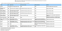 |
Table 1. Sources of bathymetry, backscatter, and seismic-reflection data used in the Vineyard and western Nantucket Sounds, Massachusetts study area. |
 |
Table 2. Confidence levels assigned to sediment texture polygons on the basis of the data used in the interpretation. The spatial distribution of polygons and associated confidence levels are shown in figure 8. |
|

