

Methodology for Construction of a Three-Layer Geologic Model of the Conterminous United States Using Land Surface, Top of Bedrock, and Top of Basement
Links
- Document: Report (11.2 MB pdf) , HTML , XML
- Data Release: USGS data release - Preliminary digital data for a 3-layer geologic model of the conterminous United States using land surface, top of bedrock, and top of basement (ver. 1.1, April 2025)
- NGMDB Index Page: National Geologic Map Database Index Page (html)
- Download citation as: RIS | Dublin Core
Acknowledgments
This study was funded by the U.S. Geological Survey National Cooperative Geologic Mapping Program. The author thanks Oliver Boyd (U.S. Geological Survey) for sharing datasets that were part of his work in building the National Crustal Model. The author credits Harvey Thorleifson (University of Minnesota) for posing the initial idea of mapping the Nation as three layers and thanks Harvey for continued thought-provoking questions on this topic.
Abstract
This report describes the methodology used for the construction of a digital three-layer geologic model of the conterminous United States by mapping the altitude of three surfaces: land surface, the top of bedrock, and the top of basement. These surfaces are mapped through the compilation and synthesis of published stratigraphic horizons from numerous topical studies. The mapped surfaces create a three-layer geologic model with three geomaterial-based subdivisions: unconsolidated to weakly consolidated sediment; layered consolidated rock strata that constitute bedrock; and crystalline rocks that are described as “basement,” consisting of either igneous, metamorphic, or highly deformed rocks. The data compilation and synthesis are highly dependent on the definition of the informal terms “bedrock” and “basement,” which may describe different ages or types of rock in different parts of the conterminous United States. This report presents the conceptualization of the three mapped layers, describes the datasets used, and summarizes the decisions made while compiling the three-layer model from the various sources. This digital dataset was created as part of efforts by the U.S. Geological Survey to develop subsurface geologic data in geospatial form as part of a broad directive to develop two-dimensional and three-dimensional geologic information at detailed, national, and continental scales. This digital dataset partly fulfills the goal of the U.S. Geological Survey’s National Cooperative Geologic Mapping Program to construct a national-scale three-dimensional geologic model.
Plain Language Summary
This report is a companion to a digital dataset created as part of U.S. Geological Survey National Cooperative Geologic Mapping Program efforts to develop subsurface geologic data in geospatial form at regional to national scales. The report describes data sources and methods used to construct a digital three-layer geologic model of the conterminous United States by mapping the altitude of three surfaces: land surface, top of bedrock, and top of basement.
Introduction
U.S. Geological Survey (USGS) science planning documents (Gundersen and others, 2011; Bristol and others, 2013) and decadal strategic plans for the USGS National Cooperative Mapping Program (NCGMP; Brock and others, 2021) call for geologic mapping across the Nation to become increasingly three dimensional (3D). The plan for nationwide 3-D geologic mapping has been endorsed by the Association of American State Geologists (Association of American State Geologists, 2014). The language in prior Congressional appropriations legislation calls for the USGS NCGMP “to bring together detailed national and continental-resolution 2-D [two-dimensional] and 3-D information produced throughout the USGS and by federal and state partners” (U.S. Congress, 2019, p. 48–49).
Compilation and synthesis of national-scale subsurface data and construction of regional-scale 3-D geologic frameworks can be aided by the construction of continuous, regional- to national-scale lithostratigraphic or chronostratigraphic surfaces that serve as datums upon which more detailed local datasets and models are built. The National Crustal Model (Boyd, 2019; Boyd and Sweetkind, 2025) uses this approach where the altitudes of a small number of major lithologic or seismic impedance boundaries are defined and used to subdivide the 3-D volume of the lithosphere. The model then uses interpolation routines to populate the volumes between these bounding surfaces using geologic map data and other data (Boyd, 2019; Boyd and Sweetkind, 202517). Definition of regionally extensive subdivisions of the subsurface is also an important part of developing a national-scale hydrogeologic framework of principal and secondary aquifers (Belitz and others, 2019). However, for a nationwide 3-D geologic model, except for regionally extensive units, such as the Trenton Limestone (or Group) in the upper Midwest or the Dakota Sandstone (or Group) of the northern Great Plains (Cohee, 1962), few named formations or lithosomes can be traced at the regional scale. As illustrated by the “Tapestry of Time and Terrain” across the contiguous United States (Vigil and others, 2000), few chronostratigraphic subdivisions are continuously traceable across the contiguous United States.
At the State level, many jurisdictions create two-layer geologic models by mapping informal units, such as depth to bedrock or depth to basement (Trotta and Cotter, 1973; Olsen and Mossler, 1982; Herzog and others, 1994; Ohio Division of Geological Survey, 2003; Hart and others, 2021). Such efforts represent achievable subsurface mapping objectives that promote the collection of new data through geophysics or drilling, foster jurisdiction-wide data compilation and interpretation, and focus effort on a specific mapping target. State geological surveys in the upper Midwest of the United States routinely produce “depth to bedrock” or bedrock topography maps where unconsolidated to poorly consolidated Pleistocene glacial deposits are of economic and civil interest because these deposits are aquifers and sources of economic sand and gravel. These deposits overlie pre-Pleistocene consolidated rocks mapped as an undifferentiated bedrock unit (Olsen and Mossler, 1982; Ohio Division of Geological Survey, 2003). The USGS has produced two-layer geologic models showing thickness of glacial materials and bedrock topography for the entire northern tier of glaciated States (Soller and others, 2012; Soller and Garrity, 2018). Similarly, basement topography maps identify the base of the stratified consolidated rock section, defining the thickness of consolidated rocks that might serve as aquifers or oil and gas targets (Frezon and others, 1983); mapping basement topography also defines the top of the prospective zone of certain types of metallic mineral deposits that may occur in undifferentiated crystalline basement rocks beneath the stratified consolidated rock section (Cole, 1976; Baranoski, 2013). The contoured top of basement rocks has been included as part of two national-scale basement maps of the United States (Basement Rock Project Committee, 1967; Bayley and Muehlberger, 1968). For the purposes of a national investigation, the question is whether there are enough local jurisdictional maps of depth to bedrock or depth to basement to compile the geomaterial layers for the entire country.
Regional- to national-scale 3-D mapping might proceed by subdividing subsurface geomaterials into three broad categories: (1) unconsolidated to poorly consolidated sediments, where units are often mapped and defined on the basis of lithology and physical properties rather than by age and stratigraphic names; (2) layered consolidated rocks, sedimentary and volcanic, consisting of mappable stratigraphic units; and (3) basement rocks, consisting of crystalline or complexly deformed rocks that cannot be treated as layers nor easily subdivided (Thorleifson, 2018, 2020, 2021; Sweetkind and others, 2021). These three geomaterials categories form a generalized three-layer model of the Nation. Model intervals are bounded by the following three surfaces: (1) land surface, (2) the top of consolidated rocks, or bedrock, which together with land surface defines the thickness of unconsolidated deposits, and (3) the top of crystalline or highly deformed rocks, or basement, which also defines the base of the section of stratified consolidated rocks (Thorleifson, 2018, 2020, 2021; Sweetkind and others, 2021). Since land surface is known, construction of a three-layer model would proceed through the definition of the top of crystalline or highly deformed rocks, or basement and the top of layered, consolidated rocks, or bedrock.
Purpose and Scope
The purpose of this study is to develop national-scale surfaces of informally named, lithologically defined interfaces within the stratigraphic column as a first step towards a national 3-D volumetric model. This report and a companion USGS digital data release (Sweetkind and others, 2024) document the results of a multiyear effort by the USGS to compile a three-layer geologic model of the conterminous United States by mapping three surfaces: land surface, the top of bedrock, and the top of basement. These surfaces are mapped through the compilation and synthesis of published stratigraphic horizons from numerous topical studies. The mapped surfaces create a three-layer geologic model with three geomaterials-based subdivisions: (1) unconsolidated to weakly consolidated sediment; (2) layered consolidated rock strata that constitute bedrock; and (3) deformed, crystalline, or metamorphosed rocks that underlie the stratified rocks and constitute basement rocks. This three-layer geologic model was created as part of efforts by the USGS to integrate and synthesize subsurface geologic data in geospatial form as part of a broad directive to develop two-dimensional (2-D) and 3-D geologic information at detailed, national, and continental scales (U.S. Congress, 2019, p. 48–49; Brock and others, 2021). The elevation, thickness, and extent of subsurface geologic units are required to define the geologic layering in any digital geologic framework model; these data, derived from previous USGS and other studies, provide a fundamental starting point. The intended uses of this dataset include national- to regional-scale resource assessments, natural resource modeling, mapping, and visualization. This USGS Data Report summarizes the conceptualization of the geologic framework, datasets used, and the methodology of construction of the three-layer model released as USGS digital data (Sweetkind and others, 2024).
Data compilation for this study was confined to the onshore part of the contiguous lower 48 States of the United States (fig. 1). This study is a map-based compilation of existing published data (Sweetkind and others, 2024); no new data or subsurface interpretations were generated to augment the existing data or extend the subsurface horizons beyond their previously published extents. Gaps in the data were allowed. There was no attempt to continue mapped horizons into areas where subsurface geology is uncertain or where little published subsurface data exist.
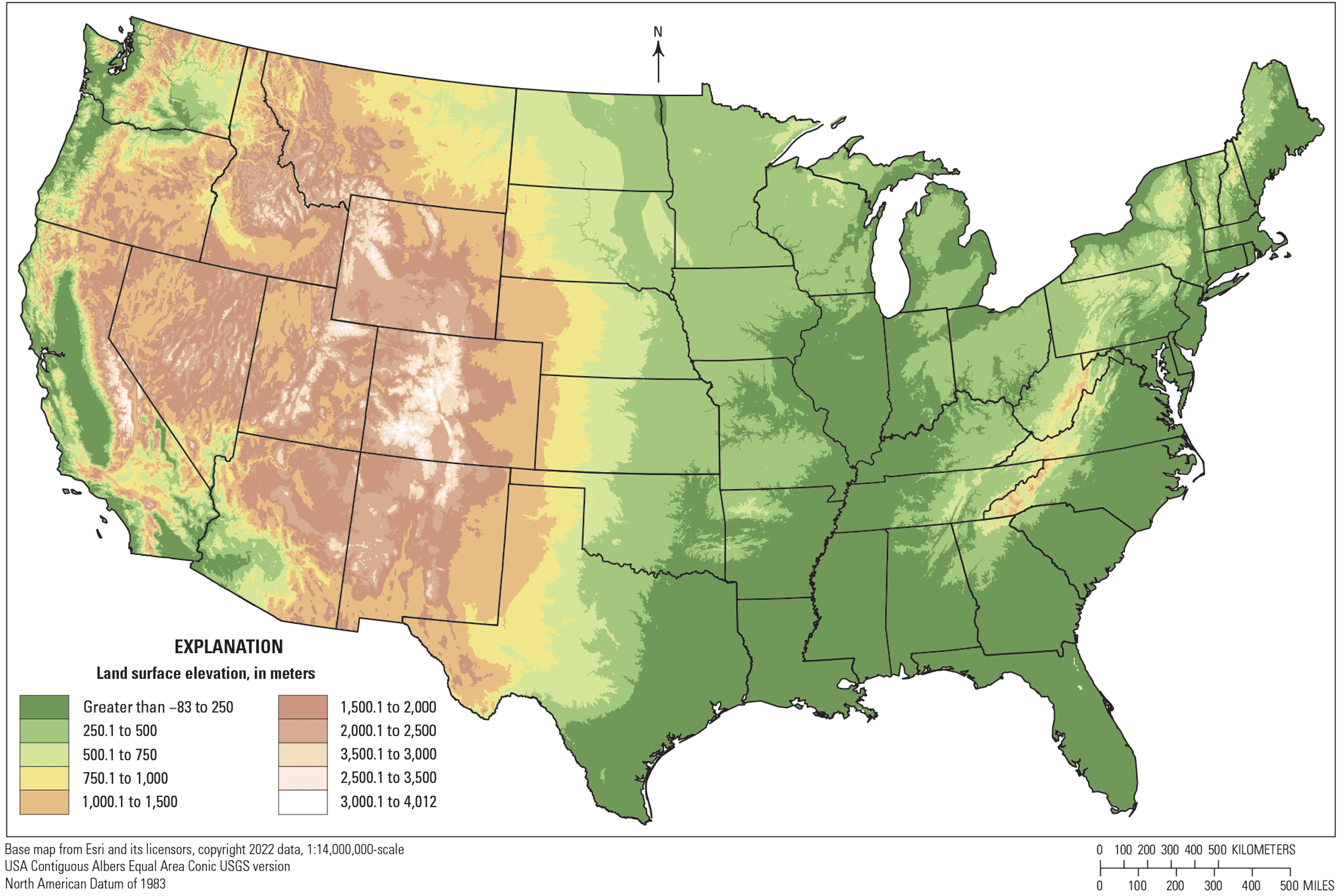
Map of the study area extent and land surface elevation of the conterminous United States at a 2.5-kilometer resolution as used in the national three-layer geologic model.
In terms of scale and spatial footprint, the three-layer geologic model of the conterminous United States presented in this report is similar to two other ongoing national-scale geologic framework projects in other USGS Mission Areas. The USGS Water Mission Area’s National-Extent Hydrogeologic Framework (NEHF) seeks to develop a consistent understanding and representation of the subsurface hydrogeology of the United States to support nationally consistent assessments of water supplies and to identify factors that affect water availability (Belitz and others, 2019). One focus of the NEHF is on compiling and extending previously mapped principal aquifers and secondary hydrogeologic regions into three dimensions. The USGS Natural Hazards Mission Area’s National Crustal Model (NCM) incorporates subsurface geology at the national scale as part of the basis for estimates of subsurface seismic velocity and density needed to improve estimates of earthquake ground shaking and seismic hazard (Boyd, 2019; Boyd and Sweetkind, 202517). The model includes lithology and age for multiple subsurface layers, including the top of bedrock, basement, lower crust, and the Moho. Each of these models is built for a specific application; all three projects have shared subsurface datasets and approaches to avoid duplication and maximize consistency.
Previous Studies
For the purposes of this study, discussion of previous regional- to national-scale subsurface mapping focuses on mapping of the depth to or altitude of two general surfaces: (1) the top of consolidated, stratified bedrock that underlies some thickness of unconsolidated surficial materials, and (2) the top of Precambrian rocks or other crystalline igneous and metamorphic rocks mapped as basement.
Bedrock Studies
Many States in the glaciated upper Midwest produce three related geologic maps: (1) surficial or Quaternary geologic maps that show the distribution and lithology of Pleistocene glacial and postglacial sediments, (2) bedrock geologic maps that map the configuration of consolidated rocks buried beneath the glacial cover, and (3) depth to bedrock maps that show the thickness of unconsolidated materials that overlie bedrock (Hart and others, 2021). Depth to bedrock maps are produced at the State and county scales (Trotta and Cotter, 1973; Olsen and Mossler, 1982; Herzog and others, 1994; Ohio Division of Geological Survey, 2003; Hart and others, 2021); such maps are used in defining potential groundwater resources in unconsolidated glacial materials and play a role in land-use planning decisions, for example, in restricting agricultural practices such as overland spreading of animal waste in sensitive areas. Regional- to national-scale maps of Quaternary sediment thickness in the previously glaciated States east of the Rocky Mountains characterize the 3-D geometry of the Quaternary sediments and buried top of consolidated rock units that lie beneath the sediments (Soller and others, 2012; Soller and Garrity, 2018, DAS13 on fig. 2 and in Sweetkind and others, 2024).
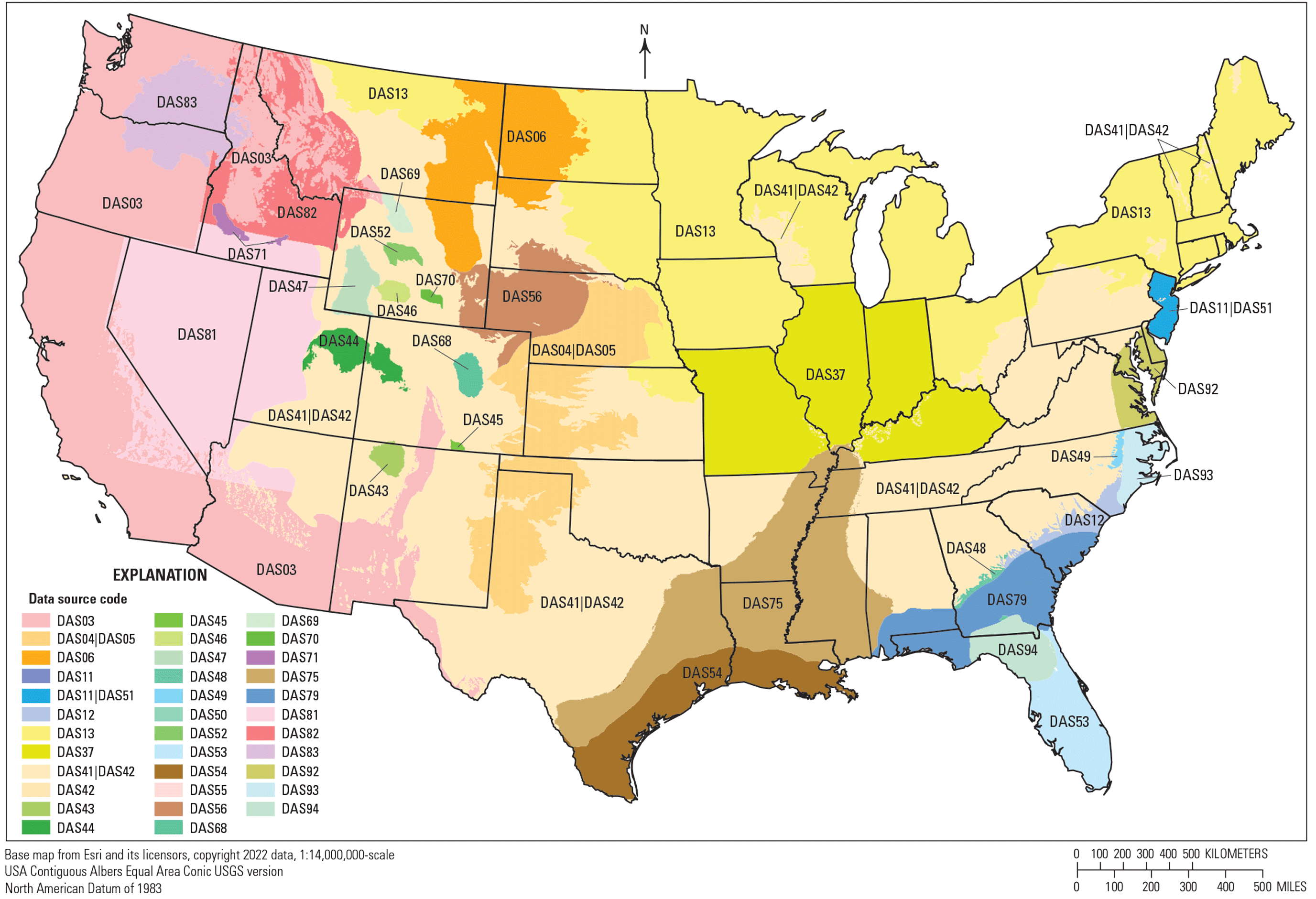
Map of data sources used to define altitude of top of bedrock of the conterminous United States in the national three-layer geologic model. Codes identifying the source of geologic data, such as DAS13, are defined in a nonspatial table in the companion digital data release that describes the sources of geologic information (Sweetkind and others, 2024).
Depth to bedrock maps are also used outside of the glaciated northern tier of States. The Arizona Geological Survey mapped the estimated depth to bedrock in Arizona, primarily using gravity methods (Richard and others, 2007). Here, depth to bedrock mapping was used to characterize the thickness of nonconsolidated Cenozoic alluvial material, which are permeable geologic materials with the potential to contain large amounts of stored groundwater. In the Arizona study (Richard and others, 2007), bedrock was defined in hydrogeologic terms as the inferred base of the basin-fill groundwater system and includes both consolidated pre-Cenozoic rocks and Cenozoic volcanic rocks that are sufficiently indurated to have low bulk permeability. The Kansas Geological Survey created a bedrock surface elevation map beneath the Ogallala part of the High Plains aquifer based on data from water and hydrocarbon wells (Macfarlane and Wilson, 2019). Bedrock was defined in the study as “Cretaceous” and “late Permian” strata that underlie the unconsolidated-to-cemented, Miocene–Pliocene deposits of the High Plains aquifer (Macfarlane and Wilson, 2019).
Gravity-based geophysical surveys in the Basin and Range Province of the Western United States take advantage of the gravity signature caused by the large density contrast between consolidated pre-Cenozoic rocks and the overlying Cenozoic sedimentary rocks that fill extensional basins (Saltus and Jachens, 1995; Blakely and Ponce, 2001). These surveys map or model the contact between low-density basin-fill deposits and the underlying more dense consolidated rocks, sometimes referred to as “basement”; gravity-based maps of the thickness of Cenozoic deposits in the Basin and Range Province are thus sometimes referred to as “depth-to-basement” maps (Saltus and Jachens, 1995; Ponce and Glen, 2008; Shah and Boyd, 2018; Florio, 2020; DAS03 on fig. 2 and in Sweetkind and others, 2024). In some of these studies, it is not clearly stated that the “basement” being referred to is the “geophysical basement,” meaning rocks that have bulk densities markedly higher than the Cenozoic basin fill, and not basement in the geologic sense of being igneous or metamorphic crystalline rocks. Use of precise terminology is important in the eastern Great Basin where Neoproterozoic and Paleozoic strata are many kilometers (km) thick and underlying crystalline rocks occur at great depths (Stewart, 1980; Hintze and Kowallis, 2009). Some gravity-based geophysical studies in the eastern Great Basin use more precise terminology to describe the stratigraphic section being modeled, distinguishing between pre-Cenozoic rocks that includes a thick Phanerozic consolidated-rock section and Cenozoic basin-fill materials (Blakely and others, 1998; Langenheim and others, 2000). A number of geologic factors affect the density based assumptions in the gravity models and add uncertainty to the fidelity of estimation of the thickness of Cenozoic basin fill, including the presence of locally thick, densely welded ignimbrites within a basin, the presence of basalts interbedded in the basin fill or localized dikes or intrusives, or the effect that the density contrast between basin fill and basement diminished with increasing depth. For the purposes of this study, gravity-based geophysical surveys in the Basin and Range Province of the Western United States more closely map the top of stratified consolidated rocks, referred to here as “bedrock,” than they map the top crystalline basement rocks.
Basement Studies
The midcontinent region of the United States is part of the cratonic platform of North America, where Proterozoic and Archean igneous and metamorphic rocks are buried beneath Phanerozoic sedimentary strata. The crystalline rocks were assembled during Proterozoic accretionary orogenies (Reed and others, 1993; Whitmeyer and Karlstrom, 2007) and subsequently affected by epeirogenic movements that produced regional-scale basins, domes, and arches (Sloss, 1988; Burgess, 2019). The thickness of the overlying Phanerozoic sedimentary strata ranges from 0 where crystalline rocks are exposed to more than 7.5 km (Frezon and others, 1983; Wandrey and Vaughn, 1997). A number of studies have delineated the inferred subsurface extent of basement domains using combinations of geological, geochemical, geophysical, and age characteristics (Sims, 1990; Whitmeyer and Karlstrom, 2007; Sims and others, 2008; Lund and others, 2015). Such studies are crucial for interpreting the history of orogenesis and the tectonic assembly of the continent (Whitmeyer and Karlstrom, 2007) and for assessing basement-rock controls on metallogenesis (Lund and others, 2015); yet none of these studies map the altitude of basement rocks beneath sedimentary cover.
Structure contours have long been a component of basement maps at a variety of scales; the contours illustrate the tectonic character and structural configuration of the cratonic platform and other areas underlain by crystalline rocks at depth (Bayley and Muehlberger, 1968; King, 1969; Muehlberger, 1992; Sims and others, 2008). Two national-scale basement maps of the United States show structure contours of basement rocks: the 1:5,000,000-scale basement map of North America (Basement Rock Project Committee, 1967) and the 1:2,500,000-scale basement rock map of the United States (Bayley and Muehlberger, 1968). Both maps show the contoured top of Precambrian igneous and metamorphic rocks of the craton but also map and contour the top of younger crystalline rocks where they are defined as “basement” in noncratonic regions. A brief description of the identity, age, and lithologic type of basement rocks is provided with the maps, but the sources of data on which the contours were drawn are not explicitly identified. At the continental scale, the King (1969) “Tectonic Map of North America” contoured the altitude of Precambrian basement rocks of the continental interior and separately showed contours of the top of Paleozoic and Mesozoic basement in the Gulf Coast region and Atlantic Coastal Plain. The Muehlberger (1992) “Tectonic Map of North America” updated and expanded on the basement map of Bayley and Muehlberger (1968), constraining the contours on the Precambrian surface with additional data from seismic-reflection profiles and borehole data. At larger map scales, regional maps of the top of Precambrian rocks have been created for the purposes of tectonic interpretation (Sims, 1990; Sims and others, 1992) and for basin-scale studies (Broadhead and others, 2009; Crain and Chang, 2018). Many State geological surveys map the depth to crystalline basement (Lawrence and Hoffman, 1993; Anderson, 1995; Hemborg, 1996).
Digital datasets for the top of crystalline basement rocks are available for only a subset of all the basement maps that have been produced. The Muehlberger (1992) “Tectonic Map of North America” has previously been available as geographic information system (GIS) data through the American Association of Petroleum Geologists, although the data were never attributed to the level required to recreate the original cartographic product. Some State geological surveys provide digital versions of their Precambrian basement maps (Wyoming State Geological Survey, 2022; University of Nebraska–Lincoln, 2025141). The National Science Foundation-funded EarthScope Ozark–Illinois–Indiana–Northern Kentucky (OIINK) experiment (Illinois State Geological Survey, 2015) compiled a digital map of the top of the Precambrian basement across four upper Midwestern States by digitizing and merging four State-scale maps. The top of Precambrian basement has been investigated at a local to regional scale to assess seismic hazard (for example, Csontos and Van Arsdale, 2008) and in carbon storage investigations (for example, Battelle, 2005; McBride and others, 2018).
The most comprehensive digital compilation of basement rock data is the digital elevation surface and digital shaded relief map of the Great Unconformity—the buried eroded top of crystalline Precambrian rocks on the cratonic platform—compiled by Domrois (2013; fig. 3A). The digital elevation surface was created through compilation and digital synthesis of State-scale contour maps showing the configuration of the Precambrian surface, augmented locally by cross section and other data (Domrois, 2013; Marshak and others, 2017a). The digital compilation of the elevation of Precambrian crystalline basement of the craton extends on the west from the west edge of the Colorado Plateau and the Wasatch Front to the Appalachian orogenic front on the east, and on the south from the edge of the Ouachita deformed belt to the U.S.–Canadian border on the north, where Precambrian rocks are exposed in the southern part of the Canadian Shield (Domrois, 2013; fig. 3A). A shaded relief image of basement topography was published with an accompanying tectonic interpretation by Marshak and others (2017b); the digital elevation surface and a table of data sources used in the digital compilation were posted to the Geological Society of America Data Repository (Marshak and others, 2017a).
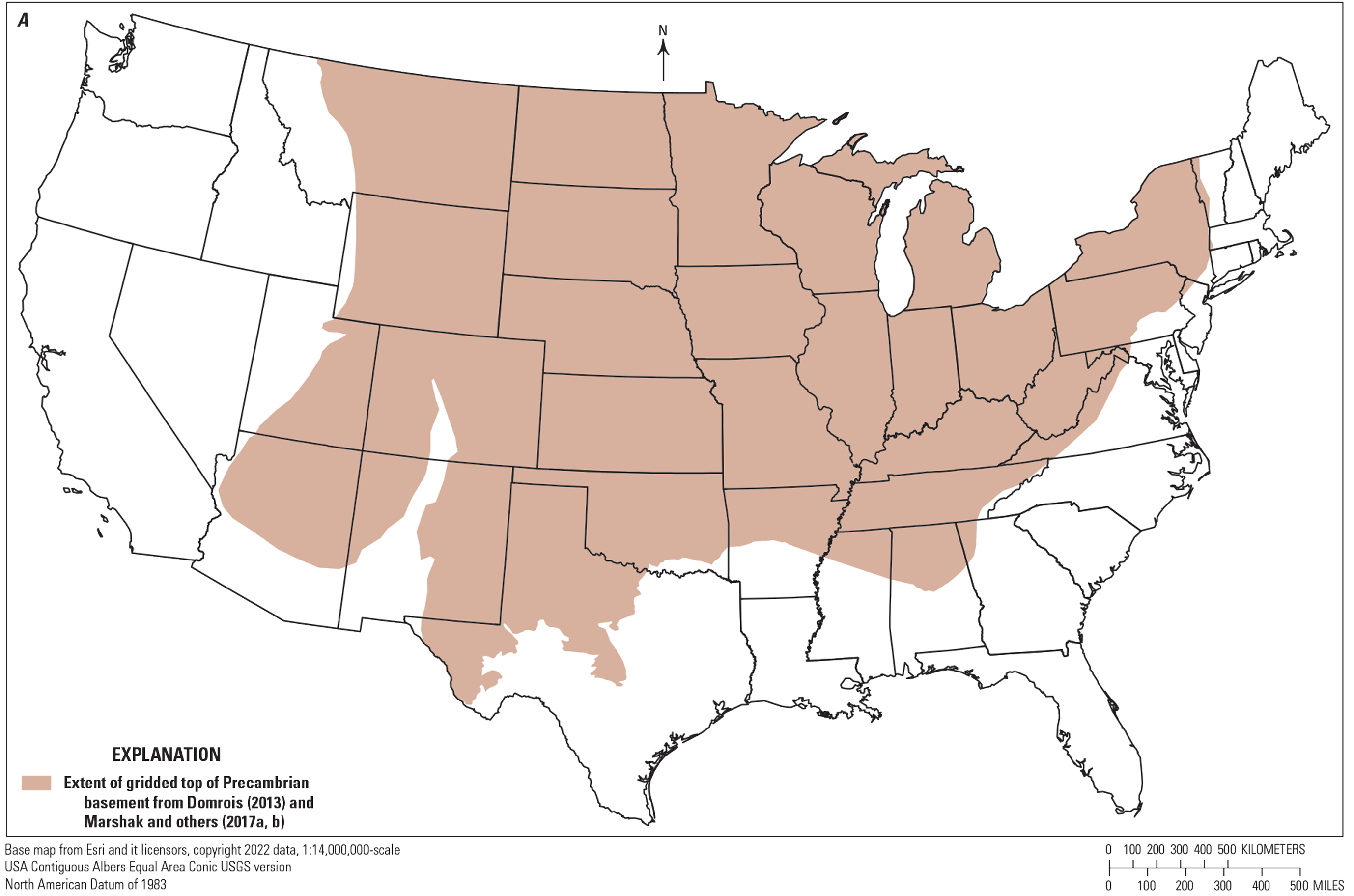
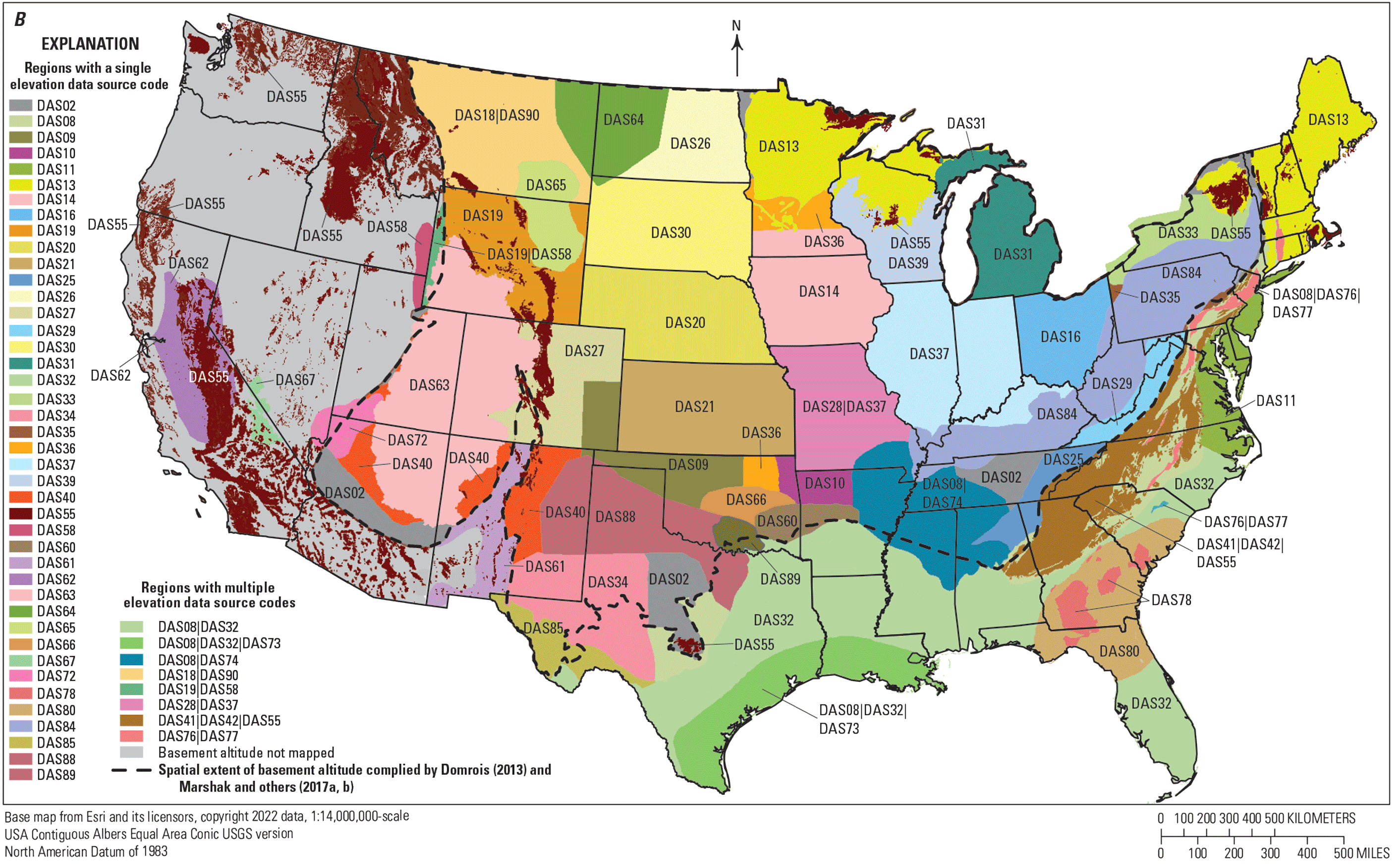
Maps of data sources used to define altitude of top of basement of the conterminous United States in the national three-layer geologic model. A, Map of the extent of the gridded top of Precambrian basement compilation of Domrois (2013) and Marshak and others (2017a, b). B, Map of other data sources used to define altitude of top of basement of the conterminous United States in the national three-layer model. Codes identifying the source of geologic data, such as DAS30, are defined in a nonspatial table in the companion digital data release that describes the sources of geologic information (Sweetkind and others, 2024). Regions where multiple data sources were used are identified with a concatenated code.
Methods
National-scale compilation of the two elevation surfaces involved searching for published reports and datasets, digitizing contours as needed, editing and attributing the elevation data, and devising a consistent series of definitions that describe the character of the unit that was being mapped.
Definition of Bedrock and Basement
Basement studies are often conducted and described without formally defining the term “basement.” None of the prior national-scale tectonic and basement maps (Basement Rock Project Committee, 1967; Bayley and Muehlberger, 1968; King, 1969) included an explicit definition of “basement.” Peter Flawn, chairman of the American Association of Petroleum Geologists Basement Rock Project Committee from 1956 to 1966, summarized the project in a keynote address at the American Association of Petroleum Geologists International Convention in 1964 (Flawn, 1965, p. 886) and ended the address by stating, “Perhaps I should have defined basement at the outset.” For the purposes of this study, basement is defined following Lund and others (2015), using the definition from the American Geosciences Institute Glossary of Geology (Neuendorf and others, 2011, p. 56), where basement is “(a) the undifferentiated complex of rocks that underlies the rocks of interest in an area. Cf: basement terrane, and (b) the crust of the Earth below sedimentary deposits, extending downward to the Mohorovicic discontinuity. In many places the rocks of the complex are igneous and metamorphic and of Precambrian age, but in some places, they are Paleozoic, Mesozoic, or even Cenozoic.” Basement rocks are thus igneous and metamorphic rocks, or highly deformed rocks, that form part of the continental crust and are often deeply buried by younger sedimentary rocks. Such rocks may be Precambrian, but particularly in the Western United States and in the Appalachian Mountains, basement rocks are younger than Precambrian.
Bedrock is defined in the American Geosciences Institute Glossary of Geology (Neuendorf and others, 2011, p. 61) as, “a general term for the rock, usually solid, that underlies soil or other unconsolidated, superficial material.” This definition works well in the previously glaciated regions of the conterminous United States, where glacial deposits overlie consolidated rocks, and in the midcontinent where neither Quaternary glacial sediments nor Cenozoic sedimentary rocks are present, and consolidated rocks underlie discontinuous surficial deposits. This definition was difficult to apply, given the time and scope of this study, to the Gulf Coast, the Atlantic Coastal Plain, intermontane basins of the Intermountain West, the Great Basin, and coastal California where unconsolidated surficial materials overlie variably consolidated older basin-fill deposits, volcanic rocks, and weakly consolidated Cenozoic sedimentary rocks. For the national-scale surface presented in this report, bedrock is defined as the base of the Cenozoic section or at a geophysically derived surface that approximates the base of the Cenozoic section. The base of Quaternary glacial sediments in the upper Midwest and the base of thin alluvial materials in the Midwest represent unique occurrences where the interface between the glacial sediments (or alluvium) and underlying Phanerozoic rocks represents the base of Quaternary, the base of Cenozoic, and the transition in material properties from unconsolidated to consolidated. Elsewhere in the United States, those three boundaries are not colocated but instead occur at separate places in the stratigraphic column. For the purposes of creating a single national-scale surface, the top of bedrock horizon is defined in this report as the base of the Cenozoic section.
Description of Data Model
The spatial data for the three-layer model released as USGS digital data (Sweetkind and others, 2024) are stored in a GIS as an array of square polygons that are 2.5 km in x and y dimensions (Sweetkind and others, 2024). Data are mapped to the x and y coordinates of the centroid of each polygon; the 2.5-km cell size thus defines the spacing between cell centroid nodes. The array of polygonal cells for the conterminous United States represents the centroids of 1,278,462 square polygonal cells. Dimensions of this cellular array are approximately 4,200 km (1,680 grid cells) in the east–west direction and 2,000 km (800 cells) in the north–south direction; the total area is approximately 8,000,000 square kilometers.
As opposed to storing surface altitude data in raster format, where an x–y coordinate pair could be assigned a single value, the three-layer model uses a two and a half-dimensional (2.5-D) approach, where surface or layer information is stored as an array of square polygons that emulate a raster layer in appearance, but each cell (or cell centroid) has a set of map coordinates and multiple descriptive attributes (Sweetkind and others, 2024). Storing data in vector-based polygonal cells allows assignment of multiple attributes at an x–y coordinate pair, including the altitude of the top of each modeled geologic unit (land surface, bedrock, and basement), the published data source from which each surface altitude was compiled, and an attribute that allows for spatially varying definitions of the bedrock and basement units. Raster layers of elevation or thickness for a unit of interest are readily exported from this cellular format. The spatial data are linked through unique identifiers to nonspatial tables that describe the sources of geologic information and a glossary of terms used to describe the method used to define the bedrock unit and the type of basement rocks being compiled (Sweetkind and others, 2024).
Data Compilation Methodology
Land surface elevation was compiled from a single source: topographic data from the National Aeronautics and Space Administration Shuttle Radar Topography Mission (SRTM; Consortium for Spatial Information, 2018). These hole-filled, seamless data were downloaded at a nominal resolution of 500-meters (m) in x and y dimensions and were resampled in a GIS to the 2.5-km cells using zonal statistics (fig. 1). These data did not include bathymetry, so only the onshore cells are accounted for.
The two subsurface interfaces within the national three-layer model (Sweetkind and others, 2024) result from the compilation of published datasets that define base of Cenozoic strata, or the “top of bedrock” (fig. 2) and base of consolidated, stratified rocks, or the “top of basement” (fig. 3). Compilation of data for the top of basement rocks began with the list of data sources published by Marshak and others (2017a) in the Geological Society of America Data Repository. The sources tabulated by Marshak and others (2017a) were confined to contoured data from the buried Precambrian craton (fig. 3A); additional searching and compilation was required to expand the dataset to other rocks considered as basement when the term is defined more broadly (fig. 3B). Data compilation for bedrock and basement surfaces was conducted using keyword searches of data repositories, including the USGS Publications Warehouse (https://pubs.er.usgs.gov/), the USGS ScienceBase Data Catalog (https://www.sciencebase.gov/catalog/), the U.S. Government’s open data website (https://data.gov/), the catalog within the National Cooperative Geological Mapping Program’s National Geologic Map Database (https://ngmdb.usgs.gov/ngmdb/ngmdb_home.html), and data that were available on the USGS Water Mission Area National Spatial Data Infrastructure node before 2023 (the data were moved from the National Spatial Data Infrastructure node website to ScienceBase in 2023).The compilation of published sources of data for the top of basement and the top of bedrock was accelerated through data-sharing as a similar compilation was being conducted in support of the USGS National Crustal Model (Boyd, 2019; Boyd and Sweetkind, 2025).
Digital data, such as grids or contour lines, were downloaded and stored in a GIS; contour maps from published reports were digitized and converted to elevation grids using standard interpolation routines within a GIS. Altitude values for each model cell were assigned by sampling the gridded input data from multiple data sources at the x and y coordinate locations of each grid node (Sweetkind and others, 2024). At every model cell, altitude of each modeled surface is compiled in meters relative to mean sea level. Altitude values were sampled from source datasets that had cell sizes ranging from 500-m to 2-km and assigned to the 2.5-km cells of the model array using statistical procedures within a GIS. Model cell values were either derived through a zonal statistics operation that calculates statistics on cell altitude values of a source raster dataset using the zones defined by the model grid, or the source dataset was converted to a triangulated surface and sampled. A mean altitude value was computed from the cells from the input raster surface whose centroids fell within a specific 2.5-km model cell. Where a unit cropped out at land surface, cells were assigned the land surface elevation. For bedrock units, where the unit was absent at the surface or in the subsurface because of erosion, the unit was assigned a null altitude value, implying a unit thickness of zero. In some regions of the model (Sweetkind and others, 2024), the basement unit was left unattributed with all attributes populated with a null value within the GIS data attributes. These were areas that had not been studied because of a lack of published subsurface data for the units of interest or lack of time and available resources in this study. Along the political boundary of the conterminous United States, the straight edges of certain model cells slightly overlap, but are mostly outside of, the curving U.S. border. These cells were left unattributed but were included in the dataset for spatial completeness (Sweetkind and others, 2024). Certain lakes within the conterminous United States had no land surface elevation assigned in the SRTM surface elevation dataset; these cells were also left unattributed and left out of subsequent model calculations.
The compiled surfaces represent horizon altitude values as derived from the individual studies without any attempt to merge or synthesize the datasets (Sweetkind and others, 2024). No attempt was made to smooth or edgematch elevation data sampled from different maps. This creates local abrupt linear discontinuities at study area boundaries.
Attributes Compiled for Modeled Surfaces
Attributes compiled for each cell of the model array of the three-layer geologic model (Sweetkind and others, 2024) include altitude of unit top, published source of the unit top altitude, an attribute “Method” for the bedrock unit that defines how the top of bedrock was defined, and an attribute “Type” for the basement unit that defines the nature of basement at the cell location. Land surface elevation is compiled with two attributes, elevation and data source; no “Type” or “Method” field is assigned to land surface elevation because the unit definition does not change across the model area.
The published source of the unit top altitude is compiled at each model cell within the digital data (Sweetkind and others, 2024); the attribute “DataSource” is a unique key to the nonspatial DataSources table that provides the full text citation and uniform resource locator (URL) for each published source dataset and a “Notes” field that provides a brief description of how the dataset was prepared for use in the model. Model cells with basement top altitudes compiled by Domrois (2013) are given two data source links—one to the basement surface compiled by Domrois (2013; fig. 3A) and a second to the original data source cited in the supplemental data sources table (Marshak and others, 2017a; fig. 3B). At the time of the Domrois (2013) compilation, some of the basement-top data were unpublished; several of the datasets have been subsequently formalized by the States and are available for download on the State websites. The cited references listed in the nonspatial DataSources table within the digital data (Sweetkind and others, 2024) are the most current (2025) version of the contoured data available, and some entries differ from the list of sources used by Domrois (2013) or in Marshak and others (2017a). All land surface elevation (fig. 1) comes from a single source (Consortium for Spatial Information, 2018; DAS01 in the DataSources table in Sweetkind and others, 2024).
The model surfaces of the top of bedrock and the top of basement are composite surfaces that are dependent on a geologic definition at any location. The attributes “Method” used for the bedrock unit (table 1; fig. 4), and “Type,” used for the basement unit (table 2; fig. 5), describe how geology is represented or aggregated within the model. Within the digital data (Sweetkind and others, 2024), each of these attributes are a unique key to an entry in the nonspatial table “Glossary” that provides a definition of the unit being mapped or, for bedrock, the method used to define the presence and altitude of bedrock units (Sweetkind and others, 2024).
Table 1.
Methods used to define top of bedrock in the conterminous United States (refer to fig. 4 for map showing locations of method use).| Bedrock method | Description of method used to define top of bedrock | References |
|---|---|---|
| BEDRX1 | Top of bedrock is top of geophysical basement as modeled from an iterative inversion of measured gravity data. Gravity data are reduced to isostatic gravity anomalies using terrain and isostatic gravity corrections. Then, the gravity field is numerically separated into two components: the field caused by higher-density consolidated rocks and the field caused by overlying less dense deposits. Mathematical inversion of basin gravity field yields an estimate of the depth to underlying dense, consolidated rocks. The density of consolidated rocks is allowed to vary horizontally, whereas the density of basin-filling deposits increases with depth according to the density-depth relations constrained with a density-depth function derived from mapped geology and drill-hole information. In the simplest geologic case in the Basin and Range where unconsolidated basin-fill alluvium overlies consolidated pre-Cenozoic rocks, the method can effectively estimate the depth to the pre-Cenozoic bedrock. Generally, density variations in the basin fill deposits, and in particular the presence of Oligocene to Miocene volcanic rocks with variable density, lead to uncertainty in the geologic identity of the gravity-derived depth-to-basement surface. | From grid of Shah and others, 2018; based on original work of Saltus and Jachens, 1995; individual gravity-based studies of Blakely and Ponce, 2001; Mankinen and others, 2004; Watt and Ponce, 2007; Ponce and Glen, 2008 were compiled into a single surface by Cederberg and others, 2011 |
| BEDRX2 | Top of bedrock is geologically defined as stratified pre-Cenozoic rocks as shown on bedrock geologic maps where the outcrops of Quaternary glacial sediments have been removed. Elevation of the top of bedrock is defined by the thickness of overlying Quaternary glacial sediments. | Soller and Garrity, 2018 |
| BEDRX3 | Top of bedrock is geologically defined as stratified pre-Cenozoic rocks that are represented on bedrock geologic maps where Quaternary cover has been removed. Elevation of the top of bedrock is defined by the thickness of nonglacial Quaternary alluvium, colluvium, and other unconsolidated deposits, as estimated by surficial geologic maps. | Soller and others, 2009 |
| BEDRX4 | Top of bedrock is geologically defined as the mapped elevation of the base of the Cenozoic section, often the top of Cretaceous rocks. Elevation of the top of bedrock is defined from borehole intercepts, structure contour maps, or surfaces derived from three-dimensional geological modeling. | Hosman, 1996; Cederstrand and Becker, 1998; Cannon and others, 2012; Thamke and others, 2014 |
| BEDRX5 | Bedrock consolidated rock units have been removed by erosion; underlying crystalline basement rocks are exposed at land surface or subcrop beneath Quaternary cover. Elevation of the top of bedrock is assigned a null value. | Surface exposures of basement rocks selected from national-scale geologic maps of Schruben and others, 1998 and Horton and others, 2017 |
| BEDRX6 | Top of bedrock primarily derived from regional maps and models of sediment thickness, combined with basin depth maps based on well data and gravity-based surveys. | From elevation grid of Shah and others, 2018, which uses the sediment model of Pelletier and others, 2016 locally modified by others studies |
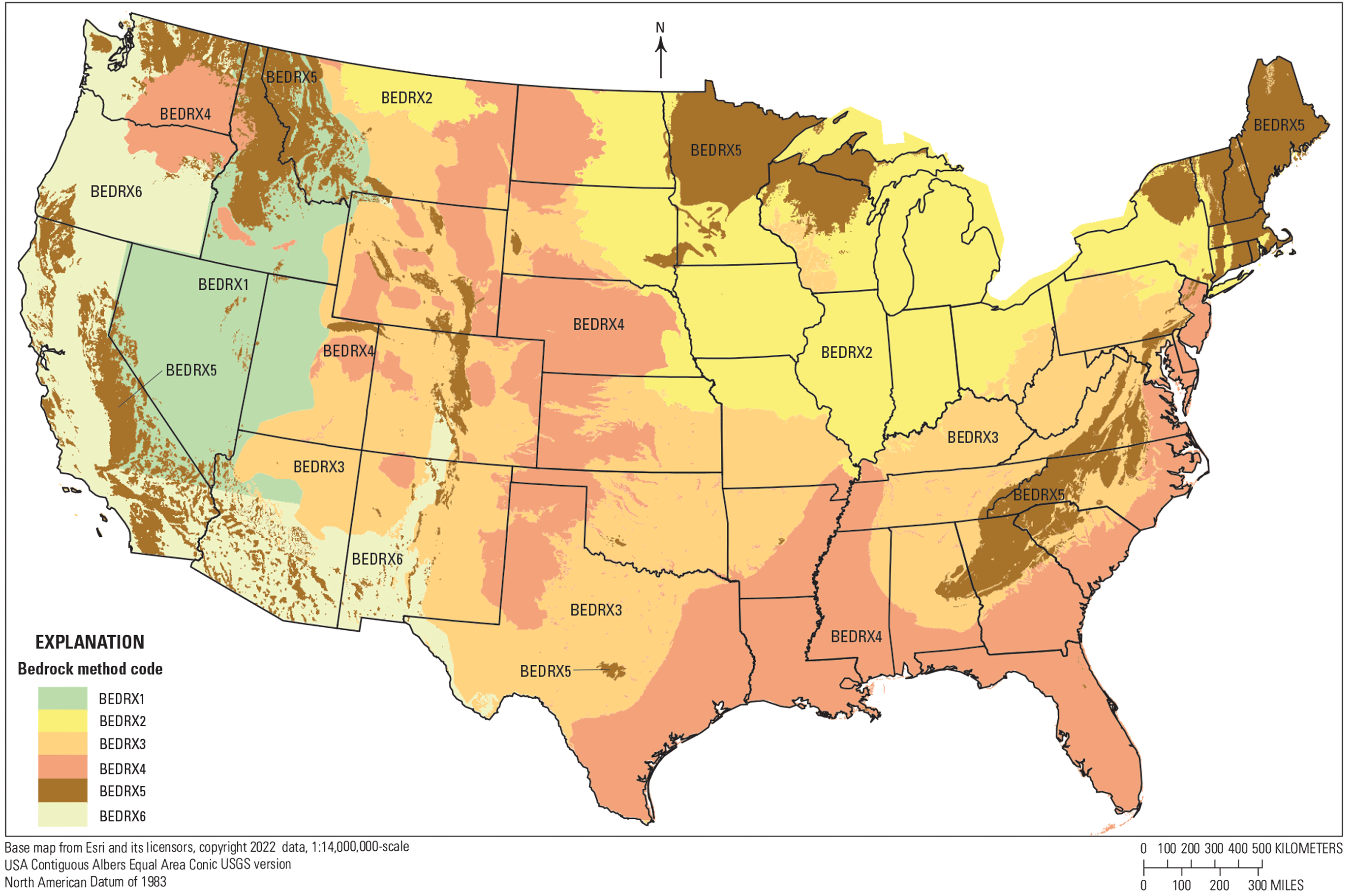
Map showing the method used to define the altitude of top of bedrock of the conterminous United States at a 2.5-kilometer resolution in the national three-layer geologic model. Bedrock method codes are defined in table 1 and in a nonspatial table in the companion digital data release that defines the terms used (Sweetkind and others, 2024).
Table 2.
Definition of basement type in the conterminous United States (refer to fig. 5 for map showing locations of basement types).| Basement type | Description of basement type | References |
|---|---|---|
| BSMT1 | Continental craton; basement surface is top of crystalline Precambrian rocks. Also includes late Proterozoic sedimentary rocks in Minnesota and the Uinta Group. | Marshak and others, 2017a; Muehlberger, 1992 |
| BSMT2 | Perimeter of Gulf Basin; basement is late Paleozoic Gondwana microcontinent (Lund and others, 2015), includes Sabine volcanic arc and Yucatan platform (Viele and Thomas, 1989). Top of basement surface is the base of the postrift Jurassic–Cretaceous rocks. | Bayley and Muehlberger, 1968; Muehlberger, 1992; |
| BSMT3 | Atlantic Coastal Plain; basement largely oceanic arc terranes of Carolinia and Charleston basement terranes (Lund and others, 2015); top of basement surface is base of postrift sediments. | Herrick and Vorhis, 1963; Muehlberger, 1992; Lawrence and Hoffman, 1993; Volkert and others, 1996; Powars and others, 2014 |
| BSMT4 | Tectonically thinned transitional crust beneath coastal parts of Gulf Coast Basin (Sawyer and others, 1991); top of basement surface is base of postrift sediments. | Sawyer and others, 1991 |
| BSMT5 | Igneous intrusive rocks—predominantly Mesozoic granitic rocks. Includes Sierra Nevada batholith, Idaho batholith, and plutons in the North Cascades. | Horton and others, 2017 |
| BSMT6 | Metamorphic rocks of various metamorphic grads and protoliths. Includes gneissic and schistose rocks of the North Cascades and in southern Montana, siliciclastic rocks of low metamorphic grade in western Montana and northern Idaho; includes crystalline Mesozoic basement beneath Cretaceous rocks of the Great Valley, including ophiolitic oceanic crust tectonically juxtaposed against Sierran basement rocks to the east, or crystalline rocks underlying Franciscan rocks of the Coast Ranges. | Horton and others, 2017 |
| BSMT7 | Basement type is unclassified. Includes highly deformed rocks and structurally intermingled rocks of various types, typically with some igneous or metamorphic component. | Horton and others, 2017 |
| BSMT8 | North American continental basement that is projected beneath folded and thrusted rocks at the leading edges of orogenic belts. | Dixon, 1982; Hatcher and others, 2007; Arbenz, 2008 |
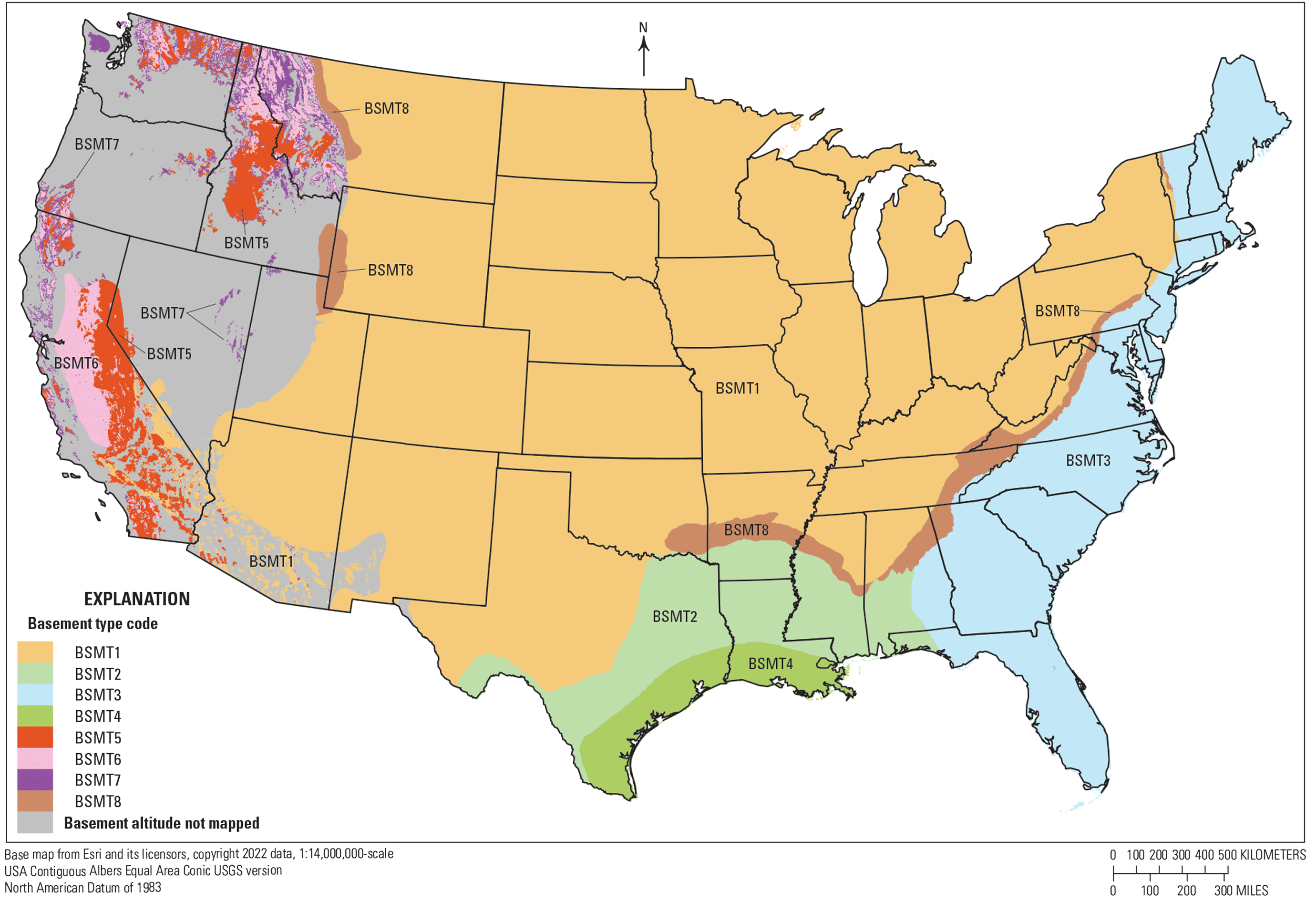
Map of the basement type for the conterminous United States at a 2.5-kilometer resolution in the national three-layer geologic model. Basement type codes are defined table 2 and in a nonspatial table in the companion digital data release that defines the terms used (Sweetkind and others, 2024).
Quality Assurance of Modeled Surfaces
Altitude values at each node within the polygonal array were evaluated for accuracy by visual inspection and a series of iterative error checks and then manually reviewed and adjusted as needed. The modeled extents of each unit were compared to the known extent of geologic units as shown on surface geologic maps and subsurface maps. Altitude and thickness values at each cell node were checked in the following ways:
-
1. The altitude of any geologic unit should be less than or equal to the land surface.
-
2. The uppermost geologic unit at any x and y coordinate must have an altitude equal to the land surface elevation.
-
3. The altitude of all geologic units must be defined at all x and y coordinates or, where not studied, a GIS null value must be present.
-
4. Geologic units cannot have negative thickness indicative of a geologic unit top crossing above the top of an overlying geologic unit.
Results
The model surfaces of the top of bedrock and the top of basement are compiled from numerous individual datasets (Sweetkind and others, 2024). Compilation results are discussed by location or geologic province below to focus on the contributions of individual data sets.
Results from Compilation of the Top of Bedrock
The national-scale top of bedrock surface compiled for the three-layer geologic model (fig. 6) is a composite surface that merges geologic horizons that are defined by different mapping methods (table 1). In the previously glaciated regions of the conterminous United States, the top of bedrock can be defined by the thickness of Quaternary glacial sediments (Soller and Garrity, 2018; bedrock method 2 labeled “BEDRX2” in fig. 4 and table 1). In the midcontinent region where neither Quaternary glacial sediments nor Cenozoic sedimentary rocks are present, the top of bedrock can be defined by the thickness of discontinuous surficial deposits (Soller and Reheis, 2004; Soller and others, 2009; bedrock method 3 labeled “BEDRX3” in fig. 4 and table 1). Where Cenozoic rocks are present along the Gulf Coast, on the Atlantic Coastal Plain, and in the Great Plains and intermontane basins of the Intermountain West, the top of bedrock is arbitrarily defined as the base of the Cenozoic section and the altitude is defined by local studies that define that horizon (bedrock method 4 labeled “BEDRX4” in fig. 4 and table 1). In part of the Western United States, the top of bedrock is defined by a gravity derived surface that approximates the base of the Cenozoic section (Saltus and Jachens, 1995; Blakely and others, 1999; Shah and Boyd, 2018; bedrock method 1 labeled “BEDRX1” in fig. 4 and table 1). Elsewhere in the Western United States, the top of bedrock is based on a model of combined sediment and soil thickness (Pelletier and others, 2016) that was modified locally through the addition of results from well data and gravity-based surveys (Shah and Boyd, 2018; bedrock method 6 labeled “BEDRX6” in fig. 4 and table 1).
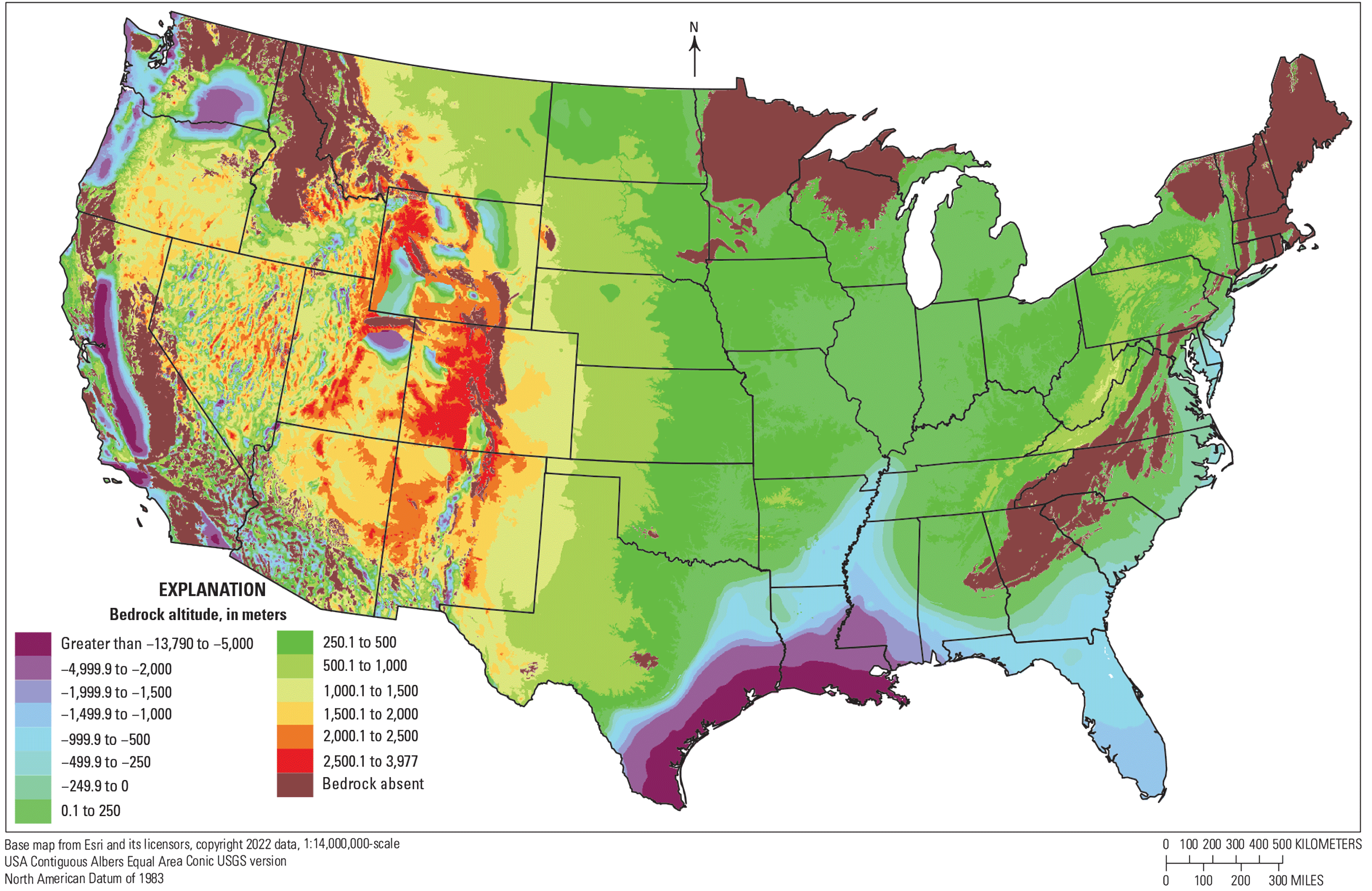
Map of altitude, in meters, of top of bedrock of the conterminous United States at a 2.5-kilometer resolution in the national three-layer geologic model. Exposures or subcrop of basement rocks where bedrock is absent is a result of erosion and the altitude of top of bedrock is assigned a null value.
Treatment of the Top of Bedrock in Previously Glaciated Regions
In the previously glaciated regions across the northern tier of States, a digital dataset of the altitude of the base of Quaternary glacial deposits (Soller and Garrity, 2018; DAS13 on fig. 2 and in Sweetkind and others, 2024) was sampled to each model cell using zonal statistics sampling in a GIS (bedrock method 2 labeled “BEDRX2” in fig. 4 and table 1). As part of their investigation, Soller and Garrity (2018) released a “Map of Bedrock Topography,” which was the altitude of the top of any consolidated rock present beneath the glacial sediments. For this study, this subsurface horizon needed to be subdivided into areas where glacial sediments overlie stratified Phanerozoic consolidated rocks that are defined as “the top of bedrock” and, where bedrock units are absent because of erosion, areas where glacial sediments overlie highly deformed or crystalline rocks defined as “basement rock units.” National bedrock geologic maps that portray the subglacial geology of the region (King and Beikman, 1974; Schruben and others, 1998; Horton and others, 2017) were used to make selection sets of map polygons of geologic units that could be classified as “bedrock” (stratified Phanerozoic consolidated rocks) or “basement” (deformed crystalline rocks of mostly Precambrian age). The selection sets were then used to guide whether the maps of Quaternary sediment thickness were used to populate the model cells for the altitude of the top of bedrock or the top of basement.
In the four-State region of Illinois, Indiana, Kentucky, and Missouri, the altitude of the buried top of bedrock surface was sampled from a digital regional map that was compiled as part of the National Science Foundation-funded EarthScope OIINK experiment (Illinois State Geological Survey, 2015; DAS37 on fig. 2 and in Sweetkind and others, 2024). That compilation itself was created by merging statewide bedrock topographic contours from Missouri, Illinois, and Indiana; in Kentucky, the EarthScope OIINK experiment used topographic data because bedrock is at or very near the surface across the State (Illinois State Geological Survey, 2015). In the previously glaciated parts of Missouri, Illinois, and Indiana, these digital data were used instead of the Soller and Garrity (2018) dataset. Quaternary sediments of the Mississippi Embayment are present in a small region in southeastern Missouri, southern Illinois, and western Kentucky; in this region, the Illinois State Geological Survey (2015) dataset was not used and instead, a contoured map of the top of Cretaceous beneath the Mississippi Embayment was used to represent the base of the Cenozoic section in this area (DAS75 on fig. 2 and in Sweetkind and others, 2024).
In the northeastern part of the Williston Basin in the northeast part of North Dakota, Cenozoic sedimentary strata underlie the Quaternary glacial sediments and overlie consolidated Cretaceous rocks that are classified as “bedrock” in adjacent areas (Thamke and others, 2014; DAS06 on fig. 2 and in Sweetkind and others, 2024). Within the basin, as much as 700 m of sedimentary rocks of the Paleogene Fort Union Formation overlie Upper Cretaceous mudstones and sandstones of the Hell Creek Formation, which overlie as much as 1,000 m of Upper Cretaceous marine shale (Gill and Cobban, 1973; Thamke and others, 2014; Spangler, 2024b). In contrast to most of the area of previously glaciated States east of the Rocky Mountains, where the base of the glacial sediments defines the altitude of the top of bedrock or, locally, the top of basement, in this part of the Williston Basin the top of bedrock is defined as the base of the Cenozoic section and the top of underlying Cretaceous consolidated rocks. Using the base of the Cenozoic section as the top of bedrock within the Williston Basin is consistent with the definition of the top of bedrock beneath the High Plains aquifer and in the intermontane basins of the Intermountain West (bedrock method 4 labeled “BEDRX4” on fig. 4 and table 1). Digital data that define the base of the Fort Union Formation (Thamke and others, 2014; DAS06 on fig. 2 and in Sweetkind and others, 2024) were sampled to define the altitude of the top of bedrock in this area.
Treatment of the Top of Bedrock Overlain by Thin Alluvial Deposits in the Midcontinent
To the south of the previously glaciated regions of the United States, bedrock units are discontinuously overlain by unconsolidated surficial deposits and weathered residuum developed on bedrock. These deposits have been mapped at a national scale, and the thickness of the deposits has been estimated (Soller and Reheis, 2004; Soller and others, 2009). Across large parts of the Central United States in areas not covered by glacially deposited sediment, these unconsolidated materials represent most or all of the thickness of sediment overlying consolidated bedrock (bedrock method 3 labeled “BEDRX3” in fig. 4 and table 1). As such, estimated thickness reported on the national compilation of surficial materials was used to estimate the altitude of bedrock in these nonglaciated regions.
The national map of surficial materials (Soller and Reheis, 2004; Soller and others, 2009; DAS41|DAS42 on fig. 2 and in Sweetkind and others, 2024) used three thickness categories that were applied to various types of surficial deposits: (1) areas where the surficial material is discontinuous or patchy in distribution, (2) areas where surficial materials are continuous in distribution and are generally less than 31-m thick, and (3) areas where surficial materials exceed 31 m in thickness. For defining the altitude of the top of bedrock, we arbitrarily assigned thickness values of 0 m, 25 m, and 50 m, respectively to the three thickness categories. In practice, a national bedrock geologic map (King and Beikman, 1974; Schruben and others, 1998) was used to identify regions where bedrock was mapped without overlying thick sections of Cenozoic sedimentary rocks, eliminating, for example, the region of the Mississippi Embayment. Within the defined regions, polygons from the national map of surficial materials (Soller and Reheis, 2004; Soller and others, 2009; DAS41|DAS42 on fig. 2 and in Sweetkind and others, 2024) were selected within a GIS, and the selected cells were assigned a thickness value based on the map unit description and published thickness classes. An altitude of the top of bedrock was calculated by subtracting the estimated sediment thickness from the DEM-derived land surface elevation (Consortium for Spatial Information, 2018). In places, thickness values were modified along alluvial drainages so that the deposits underlying the trunk stream had a greater alluvial thickness than deposits underlying tributary streams. Locally beneath map polygons of large lakes and reservoirs depicted as water, a small constant sediment thickness value was arbitrarily assigned; these polygons were depicted without an interpreted sediment thickness on the national map of surficial materials (Soller and Reheis, 2004; Soller and others, 2009; DAS41|DAS42 on fig. 2 and in Sweetkind and others, 2024).
Treatment of Top of Bedrock Beneath the High Plains Aquifer
The High Plains aquifer consists of as much as 250 m of hydraulically connected geologic units of Miocene to Quaternary age in the western part of the Great Plains in parts of Colorado, Kansas, Nebraska, New Mexico, Oklahoma, South Dakota, Texas, and Wyoming (Gutentag and others, 1984). The base of the High Plains aquifer has been mapped as part of USGS hydrogeologic studies (Cederstrand and Becker, 1998; Nebraska Water Science Center, 2016) and other studies (Macfarlane and Wilson, 2019). Across most of this region, the base of the High Plains aquifer is defined at the altitude where the Miocene–Pliocene Ogallala Formation and overlying Quaternary deposits are separated by a regional angular unconformity from underlying Permian to Cretaceous consolidated rocks (Gutentag and others, 1984). However, in the northwestern part of the aquifer extent in western Nebraska, northeastern Colorado, southwestern South Dakota, and southeastern Wyoming, Oligocene sediments of the White River Group and Arikaree Group are present between the Cretaceous rocks and the aquifer units (Gutentag and others, 1984).
For the large part of the region where the High Plains aquifer unconformably overlies Permian to Cretaceous consolidated rocks, the contoured base of the aquifer (Cederstrand and Becker, 1998; Nebraska Water Science Center, 2016; DAS04 and DAS05, respectively, on fig. 2 and in Sweetkind and others, 2024) was used to define the base of the Cenozoic section. For the northwestern part of the aquifer area where older Paleogene units underlie the Ogallala Formation, geologic map relations, a subcrop map at the base of the High Plains aquifer (Gutentag and others, 1984), and stratigraphic thickness estimates from Swinehart and others (1985) provided the conceptual framework to estimate the depth of the Mesozoic consolidated rocks beneath the contoured base of the aquifer. In this area, the altitude of the top of bedrock, defined as the base of the Paleogene section beneath the aquifer, was derived from data from a 3-D geologic model of the Denver-Julesberg Basin (Goldberg, 2025), a 3-D geologic model of the western half of South Dakota (Spangler, 2024a), and the top of the highest Cretaceous formations in oil and gas exploration boreholes in Nebraska (Nebraska Oil and Gas Conservation Commission, 2025).
Treatment of the Top of Bedrock in the Gulf Coast and Atlantic Coastal Plain
The top of bedrock in the Gulf Coast and the Atlantic Coastal Plain was taken as the base of the Cenozoic sedimentary section and top of Cretaceous rocks (bedrock method 4 labeled “BEDRX4” in fig. 4 and table 1). In the Gulf Coast, a contoured map of the top of Cretaceous from a regional stratigraphic study and aquifer analysis (Hosman, 1996; Sweetkind and others, 2023a; DAS75 on fig. 2 and in Sweetkind and others, 2024) was used for most of the onshore area; a second contoured map of the top of Cretaceous (Williamson, 1959; DAS54 on fig. 2 and in Sweetkind and others, 2024) was used for the Texas and Louisiana coastal areas. In southern Mississippi, southern Alabama, and the Panhandle of Florida, altitude of the top of the Cretaceous section was derived from contour maps of the southeastern Coastal Plain (Renken, 1996; Cannon and others, 2012). For this area, contours of the top of Navarroan rocks were used; where those rocks were mapped as absent, contours from the underlying top of Taylorean rocks were used (Renken, 1996; Cannon and others, 2012; DAS79 on fig. 2 and in Sweetkind and others, 2024).
In the Atlantic Coastal Plain, information on the altitude of the base of the Cenozoic sedimentary section and top of Cretaceous rocks came from structure contour maps of the entire Atlantic Coastal Plain (Pope and others, 2016; DAS11 on fig. 2 and in Sweetkind and others, 2024), and from more detailed local maps of the Coastal Plain in Georgia (Herrick and Vorhis, 1963; DAS48 on fig. 2 and in Sweetkind and others, 2024), North Carolina and South Carolina (Campbell and Coes, 2010; DAS12 on fig. 2 and in Sweetkind and others, 2024), Virginia (McFarland and Bruce, 2006; DAS50 on fig. 2 and in Sweetkind and others, 2024), and New Jersey (Volkert and others, 1996; DAS11|DAS51 on fig. 2 and in Sweetkind and others, 2024). Many of these maps were compiled in digital form by Mills and others (2020), which was the source of digital data used in this study.
Treatment of the Top of Bedrock in Florida
USGS hydrogeologic studies of the Floridan aquifer system that occurs in the subsurface in Florida and parts of Georgia, Alabama, and South Carolina have established the relations between regionally correlated time-stratigraphic and rock-stratigraphic units and the corresponding position of the aquifer system (Williams and Dixon, 2015; Williams and Kuniansky, 2016). The base of the Floridan aquifer system is marked by low-permeability rocks that range in age from late Eocene to late Paleocene, depending on the area considered. Throughout the Florida Panhandle, the base of the Floridan aquifer system is defined within the upper third of the Paleocene Cedar Keys Formation (Williams and Dixon, 2015; Williams and Kuniansky, 2016). The contoured base of the Floridan aquifer system (Williams and Dixon, 2015; DAS53 on fig. 2 and in Sweetkind and others, 2024) was used to approximate the base of Cenozoic surface in Florida because of the ready availability of the digital dataset and the general consistency of this horizon with adjacent base-of-Cenozoic datasets from the Atlantic and Gulf Coastal Plains.
Treatment of the Top of Bedrock in the Western United States
Regional gravity studies have long been used in the Great Basin to estimate the shape and extent of Cenozoic basins in three dimensions (Jachens and Moring, 1990; Saltus and Jachens, 1995; Blakely and others, 1999). The large density contrast between pre-Cenozoic consolidated rocks in the Great Basin and the overlying low-density Cenozoic sedimentary basin fill is used to estimate the depth of pre-Cenozoic rocks. An iterative technique separates the isostatic residual gravity anomaly into basin and basement components. Basin thickness is estimated from the basin gravity component using a density-depth relation within the basin fill (Jachens and Moring, 1990; Saltus and Jachens, 1995); the method was later modified to incorporate well and other constraints to improve the thickness estimates (for example, Blakely and Ponce, 2001).
For part of the Western United States, the altitude of the base of the Cenozoic section was derived from a gravity-based basin depth map of the Basin and Range Province (Saltus and Jachens, 1995) augmented by subsequent gravity-based studies (bedrock method 1 labeled “BEDRX1” in fig. 4 and table 1). For this study, the original basin-depth map of the Basin and Range Province (Saltus and Jachens, 1995) was modified by the results of more detailed gravity-based studies of the northern Rocky Mountains (Mankinen and others, 2004; DAS82 on fig. 2 and in Sweetkind and others, 2024), in the Death Valley region of Nevada and California (Blakely and Ponce, 2001), in eastern Nevada (Watt and Ponce, 2007), and in west-central Nevada (Ponce and Glen, 2008). The last three of these detailed datasets had been subsequently combined to support the construction of a hydrogeologic framework model of the eastern Great Basin (Cederberg and others, 2011; Sweetkind and others, 2026; DAS82 on fig. 2 and in Sweetkind and others, 2024).
One challenge of estimating the top of bedrock from gravity studies is accounting for the significant but sometimes poorly known effect that thick sections of volcanic rocks have on the density‐depth structure of the subsurface. Volcanic rocks can produce density variations that can be abrupt and unpredictable as a result of variable degree of welding in ash-flow tuffs, effects of alteration, such as zeolitization, or the presence of thick accumulations of pumiceous or nonwelded tuff. Because previous gravity-based studies may have accounted for the presence of volcanic rocks in varying ways, there is uncertainty whether the gravity defined surface within the three-layer model reliably estimates the altitude of the base of the Cenozoic section. For the National Crustal Model, Boyd (2019) suggested that the higher-density rocks that lie beneath the gravity-defined surface might include volcanic rocks older than Miocene in addition to pre-Cenozoic consolidated sedimentary rocks. This suggestion is generally consistent with the timing of eruption of widespread Oligocene to Miocene ignimbrites across the northern and central Great Basin (Best and others, 2016); these volcanic rocks would presumably be present in the deeper parts of many basins. Where a significant thickness of volcanic rocks is present within a basin, the modeled top of bedrock, defined in the model as the base of Cenozoic, might more closely represent the base of Miocene rocks, such that true bedrock could be even deeper. Another complicating factor can be the presence of basalt flows younger than Miocene within the low-density sedimentary basin fill; such basalt can cause the gravity-derived surface to be too shallow.
In parts of the Western United States outside of the extent of the gravity-based basin depth map of the Basin and Range Province (Saltus and Jachens, 1995), the altitude of the base of the Cenozoic section was derived from an elevation grid created for the crustal model of the Western United States (Shah and Boyd, 2018; Boyd, 2019; bedrock method 6 “labeled” BEDRX6 in fig. 4 and table 1). In this area, the altitude of the top of bedrock is defined by a mix of methods and is not solely gravity-based (Shah and Boyd, 2018). The base case in this area was a model of combined sediment and soil thickness derived by Pelletier and others (2016) that attempted to model the thickness of unconsolidated sediments of Miocene age or younger on a regional scale. The surface defined by Pelletier and others (2016) was modified locally by Shah and others (2018; DAS03 on fig. 2 and in Sweetkind and others, 2024) through the addition of results from well data and gravity-based surveys. However, in much of northern California, the eastern parts of Oregon and Washington, and western Idaho the altitude grid of Shah and others (2018) was unmodified from the original sediment thickness model (Pelletier and others, 2016). In these regions, the sediment thickness estimate is not based on gravity data, in contrast to the area defined as “bedrock method 1” (labeled “BEDRX1” in fig. 4 and table 1).
One challenge in the use of the elevation grid created for the crustal model of the Western United States (Shah and Boyd, 2018; Shah and others, 2018), especially for the areas where the sediment thickness model of Pelletier and others (2016) was unmodified by other data, is that a primary source for this grid, the national-scale sediment thickness map of Frezon and others (1983), did not explicitly consider or contour thickness of Cenozoic volcanic rocks in the Western United States. As a result, in areas of the Western United States where thick sections of volcanic rocks are exposed, bedrock is calculated to be at land surface. Geologically, the volcanic rocks would simply be a consolidated rock layer that would be local bedrock as distinguished from unconsolidated sediment. However, using the definitions within the three-layer model, “bedrock” is defined as the base of Cenozoic rocks, forcing the altitude of pre-Cenozoic rocks to be at land surface in areas where thick sections of Cenozoic volcanic rocks are known to exist. This is a known deficiency in the three-layer model that is not completely solved and includes areas in northeastern California, the volcanic plateaus of eastern Oregon, and parts of the northern Great Basin.
For the compilation in this study, the regional elevation surface of Shah and others (2018) was replaced locally by datasets that explicitly defined the presence and thickness of Cenozoic volcanic rocks. On the Columbia Plateau in eastern Washington, a gridded surface representing the altitude of the top of bedrock that underlies the Miocene Columbia River Basalt Group (Burns and others, 2011; DAS83 on fig. 2 and in Sweetkind and others, 2024) was used to represent the top of the pre-Cenozoic section; this forced the bedrock to a depth below the known volcanic section. In a similar way, in the western half of the Snake River Plain of southwestern Idaho, contours defining the base of basaltic volcanic rocks (Whitehead, 1992; DAS71 on fig. 2 and in Sweetkind and others, 2024) were used to approximate the base of the Cenozoic section, pushing bedrock down and allowing some part of the volcanic rock section to exist above the base-of-Cenozoic bedrock interface.
Elsewhere in the Pacific Northwest, geologic outcrop data (Colgan and others, 2011) and analysis of gravity and seismic data (Zucca and others, 1986; Khatiwada and Keller, 2015) suggest that the Cenozoic volcanic rock section is between 2–4-km thick in the region, but these topical studies provide thickness data only at points or along profiles. There is no spatially distributed dataset of the thickness of the Cenozoic section to sample as an update to the previously modeled result. Therefore, certain parts of the 3-D model are left showing pre-Cenozoic bedrock at land surface in places where geologic maps clearly show thick sections of Cenozoic volcanic rocks.
For comparison, the National Crustal Model (Boyd, 2019) adjusted for the presence of volcanic rocks in the Western United States in two ways. First, bedrock was defined as the depth to the base of unconsolidated sediment and a sediment thickness model (Pelletier and others, 2016) was modified to estimate depth to pre-Miocene strata. Second, the National Crustal Model (Boyd, 2019) estimated the top of pre-Cenozoic rocks using a map-based nearest neighbor approach that used distance to pre-Cenozoic rocks shown on regional maps. The three-layer model of this report differs substantially from the National Crustal Model (Boyd, 2019) in this area because of the differences in approach.
Top of Bedrock Data in Basins of the Rocky Mountain Region
Intermountain sedimentary basins of the Rocky Mountain region developed adjacent to basement-cored uplifts during the Laramide orogeny from latest Cretaceous through the Eocene (Baars and others, 1988; Lawton, 2008). Marine and marginal marine sedimentation associated with the intracratonic Cretaceous seaway was supplanted by deposition in continental sedimentary environments as subsiding basins received sediment shed from fault-block uplifts. Basin deposition during the Cenozoic took place in alluvial fan, fluvial, deltaic, and lacustrine settings (Baars and others, 1988; Lawton, 2008). Each of the basins of the Rocky Mountain region has a unique tectonic and basin-filling history (Baars and others, 1988; Dickinson and others, 1988), such that defining the top of “bedrock” as the base of the Cenozoic section can serve as a useful starting point to compare basin evolution in the region.
For each basin in the Rocky Mountain region (fig. 7; table 3), a published structure contour map defining the base of the Cenozoic section was georeferenced and digitized in a GIS, converted to a raster grid and elevation values were sampled to the 2.5-km array of cells (bedrock method 4 labeled “BEDRX4” in fig. 5 and table 2). For the Raton, San Juan, Greater Green River, Powder River, and Bighorn Basins, a mapped horizon that corresponded to the Cretaceous–Paleogene boundary was digitized and sampled (fig. 2; table 3; Parker, 1986; Martin, 1996; Cather, 2004; Topper and others, 2011; Thamke and others, 2014; Lynds and Carroll, 2015). For the Uinta, Piceance, Hannah, Shirley, and Laramie Basins, no published contoured horizon was available for the Cretaceous–Paleogene boundary; instead, a contoured horizon or data picked from oil and gas wells within the Upper Cretaceous section was chosen as a proxy for the base of Cenozoic (fig. 2; table 3; Larsen, 1983; Love and others, 1993; Johnson and Roberts, 2003; Wyoming Oil and Gas Conservation Commission, undated). In these basins, the vertical offset from the true elevation of the Cretaceous–Paleogene boundary was estimated from stratigraphic studies and tabulated (fig. 7; table 3). For the Wind River Basin, the best available published contour data were for a horizon within the lower part of the Paleogene section above the Cretaceous–Paleogene boundary (fig. 2; table 3; Roberts and others, 2007; DAS52). In the Denver Basin of Colorado, the Cretaceous–Paleogene boundary is exposed in outcrop at several locations around the margins of the basin (fig. 2; Dechesne and others, 2011; DAS68); to capture more of the basin geometry, the top of a deeper horizon, the Upper Cretaceous Laramie Formation (fig. 2; Dechesne and others, 2011; DAS68), was digitized (table 3).
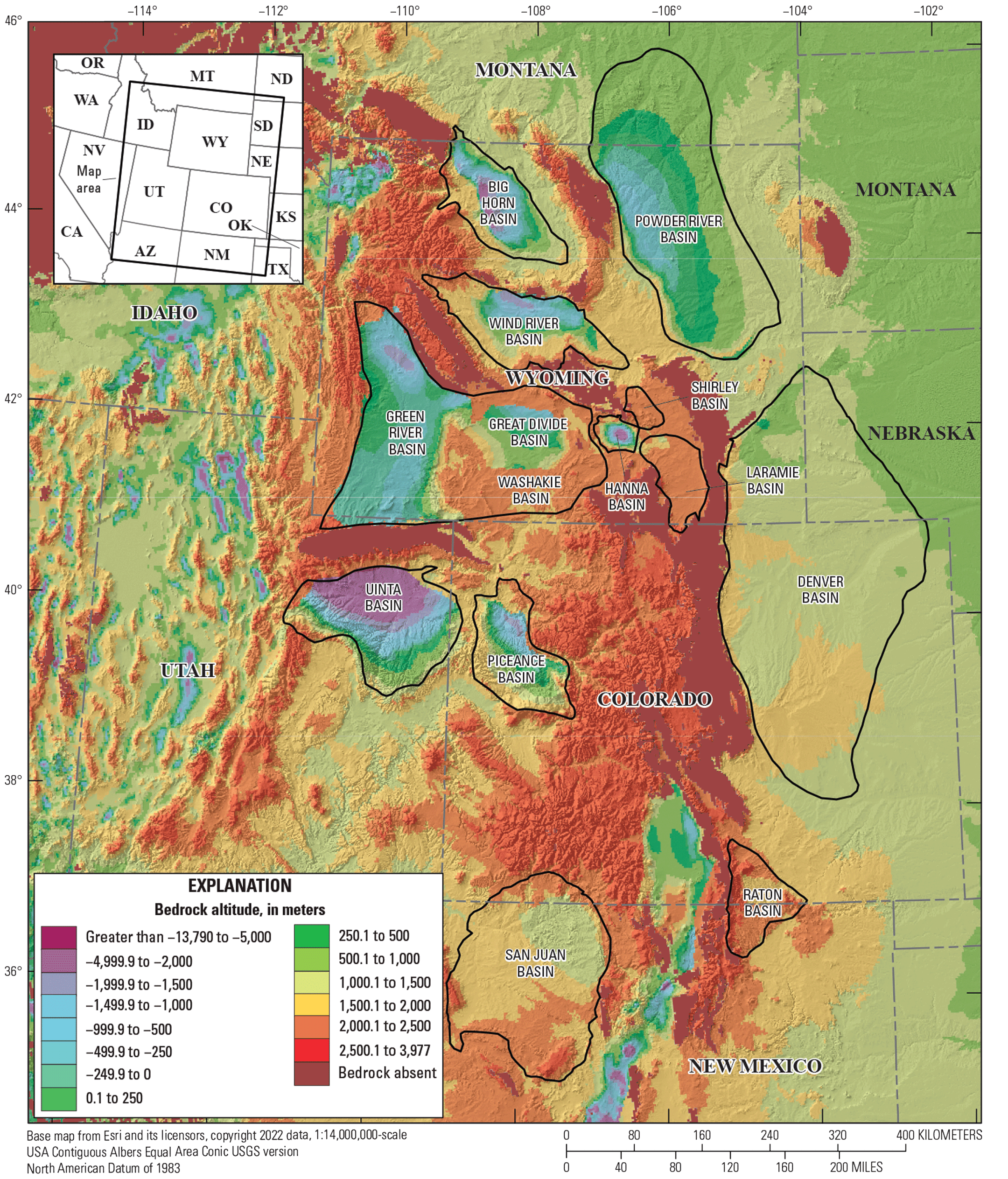
Map of altitude, in meters, of top of the bedrock and basin boundaries for sedimentary basins of the Rocky Mountain region. Basin boundaries after Coleman and Cahan (2012). Basin locations in southwestern Wyoming after Johnson and others (2011); the Greater Green River Basin mentioned in the text includes the Great Divide, Green River, and Washakie Basins.
Table 3.
Stratigraphic horizons used to approximate the base of Cenozoic section in basins of the Rocky Mountain region (refer to fig. 7 for map showing basin locations).[NM, New Mexico; CO, Colorado; m, meters; UT, Utah; WY, Wyoming; MT, Montana]
| Basin name | Horizon sampled as base of Cenozoic section | Estimated vertical offset from Cretaceous-Paleogene boundary | References1 |
|---|---|---|---|
| San Juan Basin, NM | Base of the Kimbeto Member of the Paleocene Ojo Alamo Sandstone | No offset; horizon sampled represents the K– : contact | Cather, 2004 [DAS43] |
| Raton Basin, CO | Top of the Upper Cretaceous Vermejo Formation | No offset; Vermejo Formation is uppermost Upper Cretaceous unit and its top defines the K– : contact | Topper and others, 2011 [DAS45] |
| Denver Basin, CO | Top of the Upper Cretaceous Laramie Formation | Cross sections of the Denver Basin show the top of the Upper Cretaceous Laramie Formation 100–150 m below the K– : contact, so the estimated base of Cenozoic rocks within the model generally may be too deep by that amount | Dechesne and others, 2011 [DAS68] |
| Uinta and Piceance Basins, UT and CO | Composite, time-transgressive surface merging several stratigraphic horizons near the base of the Upper Cretaceous Mesa Verde Group, including top of the Blackhawk Formation in the western part of the Uinta Basin, top of the lower part of the Castlegate Sandstone in the central and eastern parts of the Uinta Basin, and top of the Rollins Sandstone and Trout Creek Sandstone Members of the Iles Formation in the Piceance Basin | Mapped composite horizon omits the thickness of the Upper Cretaceous Mesa Verde Group, which is 500–750 m thick in most of the Uinta Basin and the western part of the Piceance Basin. The Mesa Verde Group is as much as 1,400-m thick in the deepest part of the Piceance Basin. As a result, estimated base of Cenozoic rocks within the model generally may be 500–750 m too deep and locally as much as 1,400 m too deep. | Johnson and Roberts, 2003 [DAS44] |
| Great Divide and Washakie Basins, WY, forming the eastern part of the Greater Green River Basin | Top of the Upper Cretaceous Lance Formation | No offset; Lance Formation is uppermost Upper Cretaceous unit and its top defines the K– : contact | Lynds and Carroll, 2015 [DAS46] |
| Green River Basin, forming the western part of the Greater Green River Basin, to the west of the Rock Springs Uplift, WY | Mapped horizon reported as base of Cenozoic rocks, inferred to be base of the Paleocene Fort Union Formation | No offset; horizon sampled represents the K– : contact | Martin, 1996 [DAS47] |
| Wind River Basin, WY | Base of the Paleocene Waltman Shale Member of the Fort Union Formation | Paleocene Fort Union Formation consists of two members, the Waltman Shale and a lower unnamed member. The lower member of the Fort Union thickens from less than 150 m along the south and west margins of the basin to more than 1,000 m in the deepest part of the basin. As a result, estimated base of Cenozoic rocks within the model may be 150 m to as much as 1,000 m too shallow | Roberts and others, 2007 [DAS52] |
| Powder River Basin, WY and MT | Base of the Paleocene Fort Union Formation | No offset; horizon sampled represents the K– : contact | Thamke and others, 2014 [DAS06] |
| Bighorn Basin, MT | Top of the Upper Cretaceous Lance Formation | No offset; Lance Formation is uppermost Upper Cretaceous unit and its top defines the K– : contact | Parker, 1986 [DAS69] |
| Hannah, Shirley, and Laramie Basins, WY | Top of the Upper Cretaceous Lewis Shale | Upper Cretaceous Lewis Shale is overlain by the Upper Cretaceous Fox Hills Sandstone, Medicine Bow Formation and Ferris Formation. Top of the Lewis Shale is estimated to be 1,300–2,000 m below the K– : contact, so the estimated base of Cenozoic rocks within the model may be 1,300–2,000 m too deep. | Wyoming State Geological Survey, 2022 [DAS70] |
Reference citation is followed in brackets by the DataSourceID code used in the digital dataset (Sweetkind and others, 2024) and shown on figure 2.
Treatment of the Top of Bedrock Where Basement Rocks Are Exposed at Land Surface
The altitude of the top of bedrock was assigned a null value wherever rocks defined as “basement” cropped out at land surface (bedrock method 5 labeled “BEDRX5” in table 1). National-scale geologic maps (King and Beikman, 1974; Schruben and others, 1998; Horton and others, 2017) were used to make selection sets of map polygons of geologic units that could be classified as “basement”; cells whose centroids fell within basement map polygons were assigned a null elevation value for bedrock altitude, implying that bedrock is absent in that cell.
Thickness of the Sediment Layer Between Land Surface and Top of Bedrock
The modeled thickness of the unconsolidated to weakly consolidated sediment layer was calculated as the distance between land surface and the top of bedrock (fig. 8). In areas of the conterminous United States where the bedrock unit has thickness in the model, thickness of the overlying unconsolidated sediments is calculated as the elevation of land surface minus the altitude of the modeled top of the bedrock layer. In areas where bedrock has been removed by erosion and unconsolidated deposits overlie basement rocks, the thickness of the unconsolidated sediments is calculated as the elevation of land surface minus the altitude of the modeled top of the basement layer.
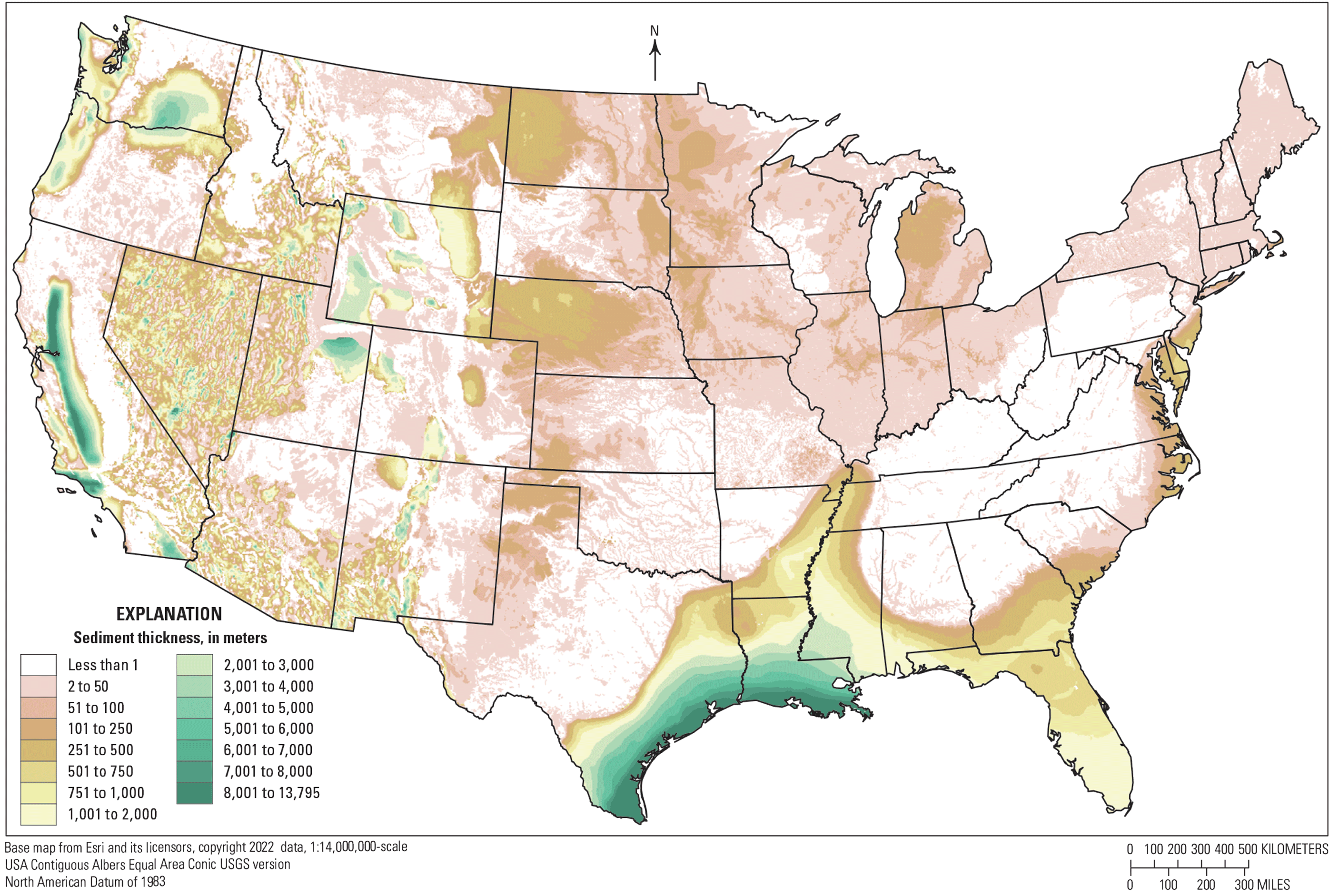
Map of the thickness of sediment for the conterminous United States at a 2.5-kilometer resolution in the national three-layer geologic model. Below 1,000 meters, the color ramp includes intermediate intervals that highlight details of distribution of relatively thin sediment.
Two first-order thickness trends are evident on the thickness of sediment map (fig. 8). One notable change in the modeled sediment thickness is caused by the change in the definition of the top of bedrock from the base of Quaternary deposits to the base of the Cenozoic. In the northern tier of previously glaciated States, where glacial deposits overlie bedrock, and in the central mid-Atlantic States and the southern midcontinent where patchy alluvial or colluvial materials overlie bedrock, the thickness of unconsolidated deposits is less than 500 m, and in many places, less than 50 m (fig. 8). In the western part of the United States, to the west of the 99th meridian (west of the north arrow; fig. 8), and in the Gulf Coastal Plain and Mississippi Embayment, the thickness of sediment calculated to the base of Cenozoic is far greater, locally resulting in a thickness of several kilometers (fig. 8). A second change in the modeled sediment thickness occurs in the Western United States at the point where the top of bedrock defined by gravity-based depth to consolidated rocks changes to a more general sediment thickness model augmented locally by other data (fig. 8; transition from the northwest corner of Nevada to eastern Oregon and northeastern California).
Results from Compilation of the Top of Basement
The national-scale top of basement surface compiled for the three-layer geologic model (fig. 9A, B) uses the approach taken by national-scale basement maps of the United States (Basement Rock Project Committee, 1967; Bayley and Muehlberger, 1968; Muehlberger, 1992) where crystalline or complexly deformed rocks of varying ages are shown on a single map. In the cratonic interior of the continent, the top of basement surface is represented by the altitude of the buried top of Archean and Proterozoic rocks, typically called Precambrian rocks in published reports (Domrois, 2013; Marshak and others, 2017b; basement type 1 labeled “BSMT1” in fig. 5 and table 2). Outboard of the craton, igneous, and metamorphic rock complexes that underlie layered Phanerozoic rocks are routinely referred to as “basement” in the Gulf Coast (Sawyer and others, 1991; basement types 2 and 3 labeled “BSMT2” and “BSMT3” in fig. 5 and table 2), the Atlantic Coastal Plain (Murray, 1961; basement type 3 labeled “BSMT3” in fig. 5 and table 2), and even in California (Wentworth and others, 1995; basement type 6 labeled “BSMT6” in fig. 5 and table 1). Within the GIS dataset for the three-layer geologic model, an attribute “Type” is used to define and distinguish among the various usages of the term basement (table 2; Sweetkind and others, 2024).
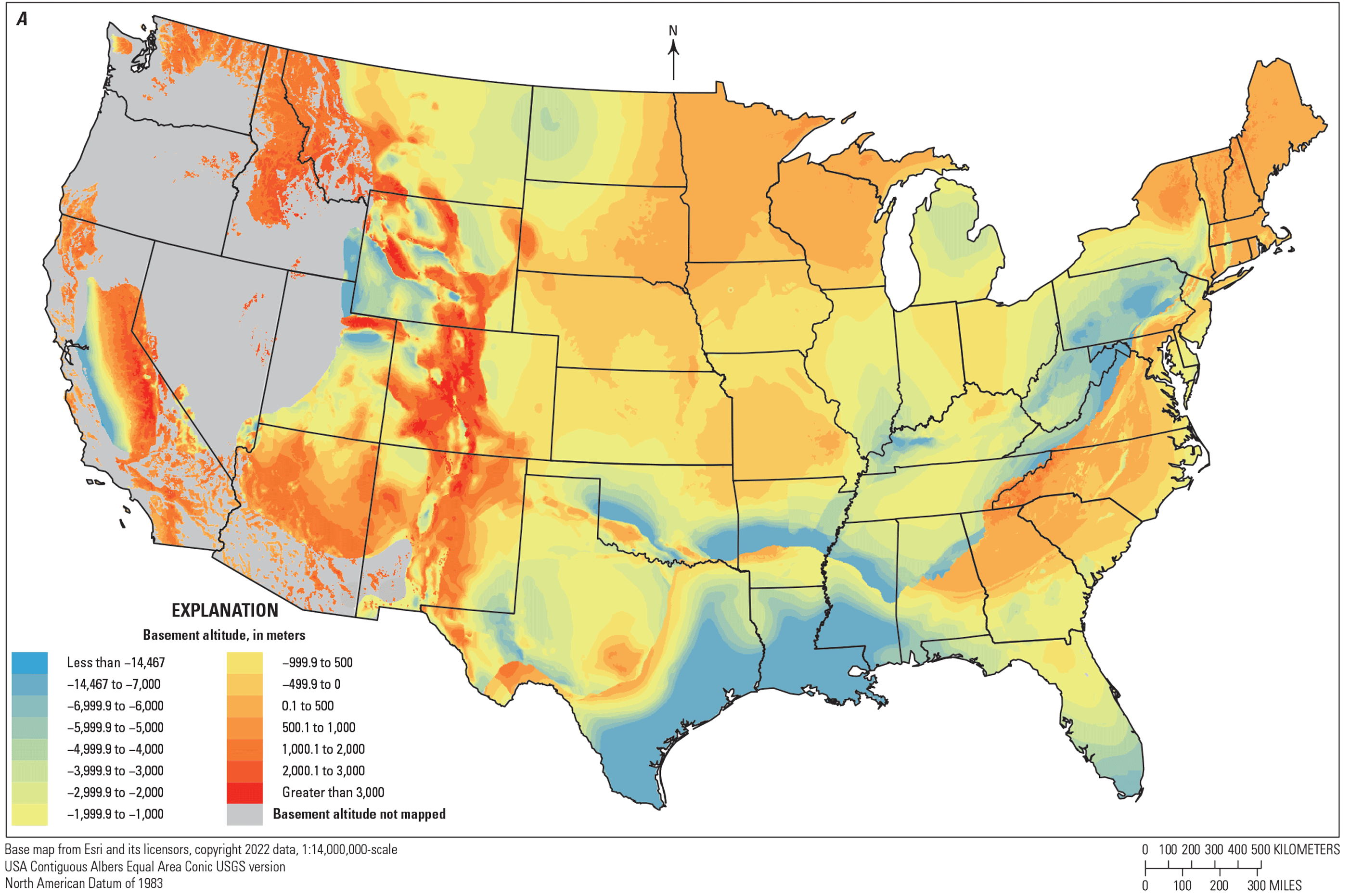
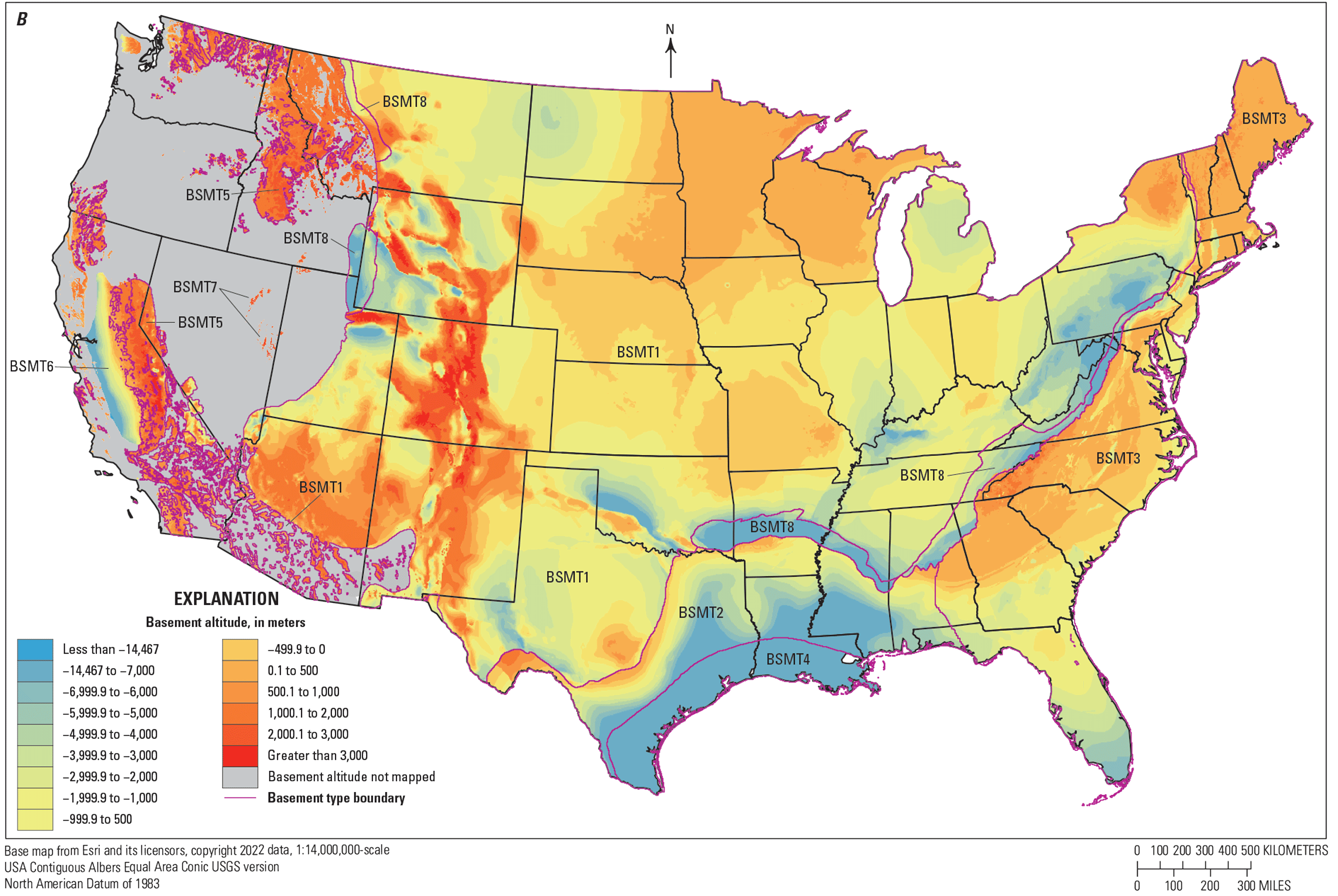
Maps of the altitude of the top of basement A, without basement type codes and B, with basement type codes labeled in the conterminous United States at a 2.5-kilometer resolution in the national three-layer geologic model. Gray areas in the Western United States are where the altitude of basement was not mapped.
Crystalline basement of probable Proterozoic age has long been inferred to exist in the subsurface of the Western United States as far west as central Nevada, approximately at long 116° W (Levy and Christie-Blick, 1989; Whitmeyer and Karlstrom, 2007; Lund and others, 2015). The subsurface presence of basement rocks with continental affinities has been inferred on the basis of continental seismic-reflection profiling (Allmendinger and others, 1987), deep crustal magnetotelluric soundings (Wannamaker and Doerner, 2002; Grauch and others, 2003), and isotopic data (Bennett and DePaolo, 1987; Tosdal and others, 2000). Inclusion of basement rock data for the present three-layer model compilation requires a published map of basement altitudes, not just the inferred presence of basement rocks at depth. As such, the top of basement mapped in this study ends in west-central Utah and southernmost Nevada, the most westerly locations where published altitude data for buried Proterozoic rocks were found (fig. 9A, B). Throughout northwestern Utah, much of Nevada, northern California, Oregon, and Washington, the altitude of the top of basement has not been mapped and there is a data gap in the top of basement surface, except where basement altitude is controlled by outcrops of crystalline rocks that are mapped at land surface on geologic maps (fig. 9A, B).
Treatment of the Top of Basement for the Craton in the Midcontinent
The digital elevation surface of the top of crystalline Precambrian rocks on the cratonic platform (Domrois, 2013; Marshak and others, 2017a; fig. 3A) was the starting point for the compilation of basement rock data for this study. The digital raster data and table of map sources were downloaded (Marshak and others, 2017a), data were reprojected to a preferred coordinate system, and altitude values of the Precambrian surface were converted from feet to meters. The published top of Precambrian surface was locally edited to remove minor elevation errors, resampled to the 2.5-km grid used in this study, and, where geologic maps showed Archean or Proterozoic rocks at land surface (Schruben and others, 1998; Horton and others, 2017), the altitude values of the sampled surface were adjusted to match the land surface elevation grid used in this study. The digital elevation surface of Marshak and others (2017a; fig. 3A) was compared to statewide maps showing the altitude of the top of Precambrian rocks that were sources for the Marshak and others (2017a) compilation, including Wyoming (Wyoming State Geological Survey, 2022; DAS19 on fig. 3B and in Sweetkind and others, 2024), Colorado (Hemborg, 1996; DAS27 on fig. 3B and in Sweetkind and others, 2024), Kansas (Cole, 1976; DAS21 on fig. 3B and in Sweetkind and others, 2024), Iowa (Anderson, 1995; DAS14 on fig. 3B and in Sweetkind and others, 2024), and Ohio (Baranoski, 2013; DAS16 on fig. 3B and in Sweetkind and others, 2024). In all these cases, the regional “basement” compilation (Marshak and others, 2017a; DAS02 on fig. 3B and in Sweetkind and others, 2024) correctly represented the data shown on the source maps. As compilation of altitude data from areas surrounding the cratonic platform progressed, some of the outlying regions of the Marshak and others (2017a) elevation surface were edited for consistency with other input data discussed in this report.
The compiled top of crystalline Precambrian rocks of the continental interior (Domrois, 2013; Marshak and others, 2017a, b; fig. 3A) was modified and locally extended for the current (2025) compilation using cross section data or contoured data from numerous published reports (fig. 3B). A raster surface for the top of Precambrian was created for the four-State region of Missouri, Illinois, Indiana, and Kentucky as part of regional EarthScope OIINK research on the tectonics of the midcontinent (Illinois State Geological Survey, 2015; DAS37 on fig. 3B and in Sweetkind and others, 2024). The source maps used for the four-State compilation are the same as those maps used by Domrois (2013) and subsequent reports for the craton-wide compilation. For this report, the data from the four-State compilation (Illinois State Geological Survey, 2015) were used in this region because these data were created with direct involvement of the four State geologic surveys and are presumed to be the authoritative dataset for this region. A structure contour map of the top of Precambrian rocks in the upper Midwest developed by the Midwest Regional Carbon Initiative helped to refine basement elevations and the presence of the Rome Trough beneath the Appalachian Basin (Battelle, 2005; DAS84 on fig. 3B and in Sweetkind and others, 2024). To the west and southwest of the Permian Basin in west Texas, published contour maps of the top of Precambrian rocks (Hills, 1984; Bureau of Economic Geology, 2009; both are shown as DAS34 on fig. 3B and in Sweetkind and others, 2024 and Shuster and others, 2021; DAS85 on fig. 3B and in Sweetkind and others, 2024) were digitized and sampled to extend the compiled top of crystalline Precambrian rocks of the continental interior (Domrois, 2013; Marshak and others, 2017a, b) farther to the west.
The published basement compilation of Marshak and others (2017a, b) extends only to the eastern front of the Idaho-Wyoming thrust belt in western Wyoming (fig. 3A), although the top of Precambrian rocks is interpreted as dipping westward beneath the thrust belt in relatively undeformed fashion (Dixon, 1982; Wyoming State Geological Survey, 2022). Data on the altitude of the Precambrian surface beneath the Idaho-Wyoming thrust belt in western Wyoming came from a digital version of the structure contours shown on the Precambrian basement map of Wyoming (Wyoming State Geological Survey, 2022; DAS19 on fig. 3B and in Sweetkind and others, 2024) and from altitude points measured from published serial geologic cross sections drawn across the thrust belt (Dixon, 1982; DAS58 on fig. 3B and in Sweetkind and others, 2024). Structure contour and point data were combined in a GIS, interpolated to a raster surface, and the result was sampled to the 2.5-km cells for this study.
The published basement compilation of Marshak and others (2017a, b; fig. 3A) did not include elevation data from within the Rio Grande Rift in New Mexico or Colorado, although contour maps of the top of Precambrian in New Mexico (Broadhead and others, 2009; DAS61 on fig. 3B and in Sweetkind and others, 2024) and Colorado (Hemborg, 1996; DAS27 on fig. 3B and in Sweetkind and others, 2024) show contours for some areas within the rift. The Colorado map (Hemborg, 1996) was georeferenced in a GIS and the contours digitized and combined with digital contour data of the top of Precambrian in New Mexico (Broadhead and others, 2009); contours were interpolated to a raster surface, and the result was sampled to the 2.5-km cells for this study.
The compiled top of crystalline Precambrian rocks of the continental interior (Domrois, 2013; Marshak and others, 2017a, b; fig. 3A) was modified using the modeled top of Precambrian rocks from several published 3-D geologic models. The modeled top of Precambrian surface from digital 3-D geologic models of the Williston Basin in Montana, North Dakota, and South Dakota (Gelman and Johnson, 2023; Spangler, 2024b; DAS64 on fig. 3B and in Sweetkind and others, 2024) and the Powder River Basin in Wyoming and Montana (Spangler and others, 2023; Spangler, 2024b; DAS65 and DAS91, respectively, on fig. 3B and in Sweetkind and others, 2024) was extracted from the published datasets, manipulated in a GIS, and sampled to the 2.5-km cells. Elevation data for the top of Precambrian rocks beneath the Colorado Plateau were sampled from the top of a hydrogeologic unit contained within a 3-D hydrogeologic model of the Upper Colorado River Basin in New Mexico, Arizona, Utah, Colorado, and Wyoming (Sweetkind and others, 2023b). In the published hydrogeologic model, the deepest hydrogeologic unit combined altitude data from Precambrian basement rocks and Cenozoic intrusive rocks to model the crystalline rocks at the base of the aquifer system (Sweetkind and others, 2023b; DAS63 on fig. 3B and in Sweetkind and others, 2024). This horizon was extracted from the published dataset, and model cells associated with Cenozoic intrusive rocks were identified by comparison with regional geologic maps (Schruben and others, 1998; Horton and others, 2017). Model cell altitude values were manually edited to remove land surface elevations or altitudes in the shallow subsurface that represented outcropping or near-surface intrusive bodies; altitude values were replaced by values that represented a local average altitude for Precambrian rocks adjacent to the modeled intrusive body. These revised data were then sampled to the 2.5-km cells for this study. A digital hydrogeologic model of the Death Valley regional flow system in Nevada and California (Faunt, 2006, Faunt and others, 2010; DAS67 on fig. 3B and in Sweetkind and others, 2024) included a model unit called the crystalline confining unit that represented the altitude of crystalline Precambrian rocks at the base of the groundwater flow system. Altitude data for the crystalline confining hydrogeologic unit were selected from the western parts of the model, near and to the west of the Death Valley fault zone, where Precambrian rocks crop out or are inferred in the subsurface in the Funeral Mountains, the Panamint Range, and surrounding region (Sweetkind and others, 2001; Workman and others, 2002). The selected model data were manipulated in a GIS and sampled to the 2.5-km cells.
Treatment of the Top of Basement Surface in the Ouachita-Marathon Orogenic Belt and Gulf Coast Region
Basement rocks of the Gulf Coast region lie to the south of the Ouachita-Marathon orogenic belt that forms the northern and northwestern flank of the Gulf of Mexico Basin (Viele and Thomas, 1989; Poole and others, 2005; Snedden and Galloway, 2019). In general, Proterozoic basement rocks of the Gulf Coast region are considered to have Gondwanan affinities (basement type 2 labeled “BSMT2” in fig. 5 and table 2) and were added to the margin of the continent during a late Paleozoic collisional-subductional event (Viele and Thomas, 1989; Lund and others, 2015; Ewing and others, 2019). These rocks were subsequently subjected to rifting and crustal attenuation (basement type 4 labeled “BSMT4” in fig. 5 and table 2) during the Late Triassic to Early Jurassic during the breakup of the supercontinent Pangea, resulting in a south-to-southeastward transition from crust with continental affinities to oceanic crust (Worrall and Snelson, 1989; Sawyer and others, 1991; Snedden and Galloway, 2019) that is now deeply buried by coastal plain sediments and rock strata.
National-scale tectonic and basement maps of the Gulf Coast region show the structural configuration of basement rocks at the base of the postrift Mesozoic marine section (Sawyer and others, 1991; Muehlberger, 199290). Knowledge of the depth to basement in the Gulf Coast region come from onshore wells around the margins of the basin that penetrate, and sometimes sample, the basement rocks and from wells that penetrate deeply into the sedimentary section without encountering basement, which provide a minimum constraint on basement depth (Sawyer and others, 1991; Snedden and Galloway, 2019). Most of the knowledge of depth to basement from the water-covered areas of the central and southeastern Gulf of Mexico Basin comes from seismic-reflection profiles that image basement (Sawyer and others, 1991; Snedden and Galloway, 2019).
For this study, the altitude of basement rocks to the south of the Ouachita-Marathon orogenic belt in the Gulf Coast region was compiled from digital contour data served by the American Association of Petroleum Geologists for the Tectonic Map of North America (Muehlberger, 1992; DAS32 on fig. 3B and in Sweetkind and others, 2024). This map included data from seismic-reflection profiles and well data to constrain the location of contours on the basement surface and was used in preference to older national-scale tectonic maps (Basement Rock Project Committee, 1967; Bayley and Muehlberger, 1968; King, 1969). For the immediate onshore part of the Gulf Coast, the contoured base of the Mesozoic marine section, (Sawyer and others, 1991; DAS73 on fig. 3B and in Sweetkind and others, 2024) were used to augment the basement contours shown on the Tectonic Map of North America (Muehlberger, 1992). Basement contours shown on the King (1969) tectonic map were notably shallower than other basement maps of the region. For example, near Houston, Texas, the King (1969) map shows the altitude of basement at about −3,000 m, whereas the map of Sawyer and others (1991) shows the altitude of basement at about −11,000 m and Muehlberger (1992) maps the top of basement at about −9,750 m. Along the Texas coastline, King (1969) maps the top of basement at −3,800 m, whereas Sawyer and others (1991) map the altitude of basement close to −11,000 m and Muehlberger (1992) maps the top of basement at about −12,000 m. The basement structure contours from King (1969) were not used in this study because the more recent tectonic maps (Sawyer and others, 1991; Muehlberger, 1992) are generally much deeper and are consistent with each other.
Along the north edge of the Ouachita-Marathon orogenic belt, the Proterozoic crust of the North American craton is obscured by, and possibly involved in, Pennsylvanian to Permian thrust sheets in a broad, arcuate belt that extends from the southeastern end of the Appalachian Mountains to the Marathon region of west Texas (Viele and Thomas, 1989; Ewing and others, 2019). Where subsurface data are plentiful, Proterozoic crystalline rocks may be projected beneath the allochthonous rocks of the orogenic belt (basement type 8 labeled “BSMT8” in fig. 5 and table 2). For the Ouachita Mountains, Arbenz (2008) created a suite of serial cross sections that portrayed the subthrust geometry and interpreted altitude of Precambrian basement beneath the thrusts. The change in basement definition from Precambrian basement of the craton to the basement rocks of the Gulf Coast region was arbitrarily taken as the point at which Precambrian basement of the craton was overlapped by the first thrust faults that involved highly deformed Cambrian forearc rocks (Arbenz, 2008). This created an abrupt elevation discontinuity across the orogenic front where two differently defined basement blocks are juxtaposed (fig. 9A, B).
Treatment of the Top of Basement in the Appalachians and Atlantic Coastal Plain
Metamorphic rocks of various grades form the crystalline, interior parts of the Appalachian orogenic belt (Hatcher, 1989); these rocks are defined as “basement” for the purposes of this study (basement type 3 labeled “BSMT3” in fig. 5 and table 2). These rocks crop out in northern Georgia, western North Carolina and South Carolina, western Virginia, and western Maryland (Hatcher, 1989; Horton and others, 2017). Basement rocks in this region were selected using the lithologic descriptor attributes in the Horton and others (2017) digital geologic map dataset; metamorphic rock names and metasedimentary and metaigneous lithologic descriptors were selected from the attribute table of the geologic polygons. The selection set from the geologic map was compared to the type and thickness of mapped surficial cover (Soller and Reheis, 2004) to confirm that the metamorphosed rocks were at or very near land surface. The top of basement altitude was then calculated for each 2.5-km cell using land surface elevation derived from a DEM.
The top of the basement surface beneath the southern Appalachian foreland fold and thrust belt has been constructed by combining data from seismic-reflection profiles, geologic maps, and well data (Hatcher and others, 2007; basement type 8 labeled “BSMT8” in fig. 5 and table 2). The eastward change in basement definition from the subthrust Archean to Proterozoic basement of the craton (basement type 8 labeled “BSMT8” in figs. 7B and 8) to crystalline rocks of the Blue Ridge–Piedmont crystalline sheet (basement type 3 labeled “BSMT3” in figs. 7B and 8; Hatcher and others, 2007) was arbitrarily chosen at the point where cratonic crust of the continental interior is overlapped in map view by younger, continent-vergent basement rocks. As a result of the change in definition, the mapped basement surface has a large and abrupt change in elevation at the orogenic front (fig. 9A, B).
The altitude of the top of the basement rocks of the Appalachian orogen that are buried beneath the Atlantic Coastal Plain (basement type 3 labeled “BSMT3” in fig. 5 and table 2) initially came from digital structure contours shown on the “Tectonic Map of North America” (Muehlberger, 1992; DAS32 on fig. 3B and in Sweetkind and others, 2024). These data were subsequently modified by data from regional studies that mapped the sub-Coastal Plain basement rocks in the Southeast Coastal Plain in northern Florida, southeastern Georgia, southeastern South Carolina (Murray, 1961; Mills and others, 2020; DAS80 on fig. 3B and in Sweetkind and others, 2024), and on the northern Atlantic Coastal Plain (Pope and others, 2016; DAS11 on fig. 3B and in Sweetkind and others, 2024).
Deformed and metamorphosed basement rocks of the Appalachian chain are disrupted by Late Triassic to Early Jurassic rift basins, which contain locally thick accumulations of continental siliciclastic, lacustrine, and basaltic rocks. The altitude of the underlying basement may be as much as several kilometers deeper than similar rocks on the margins of the rift basins (Manspeizer and others, 1989; Schlische, 1993; Withjack and others, 2012). Faults and geologic polygons from the geologic compilation of Horton and others (2017) were used to locate the basins in map space; basement rock altitudes from the basement rock map of the United States (Bayley and Muehlberger, 1968; DAS08 on fig. 3B and in Sweetkind and others, 2024) were digitized to initially construct basement depth with the rift basins. Data from geologic cross sections and seismic-reflection profiles were used to refine basin depth and polarity (Manspeizer and others, 1989; Schlische, 1993; Withjack and others, 2012; DAS76 and DAS77 on fig. 3B and in Sweetkind and others, 2024). Basement rock altitudes within the South Georgia Rift basins were derived from a contoured figure in Heffner (2013; DAS78 on fig. 3B and in Sweetkind and others, 2024).
Use of Geologic Maps to Add the Top of Basement from Outcrops in the Western United States
Basement maps of the conterminous United States include Mesozoic and Cenozoic batholithic intrusive bodies of the Western United States cordillera. Basement Rock Project Committee (1967) map these rocks as “acid and intermediate plutonic rocks”; Bayley and Muehlberger (1968) subdivided major intrusive rock bodies into broad compositional and age classes, and, using color tones on the map, distinguishing between exposed rocks and subsurface rocks that were known or inferred from drill holes or projection of outcrop.
Major intrusive rock bodies in the Western United States were selected using the lithologic descriptor attributes in the Horton and others (2017) digital geologic map dataset. Igneous rock names and lithologic descriptors, such as granite, granodiorite, tonalite, quartz diorite, quartz monzonite, and others, were selected from the attribute table of the geologic polygons (basement type labeled “BSMT5” in fig. 5 and table 2). Smaller intrusive bodies, generally smaller than 250 square kilometers in area, were removed from the selection set; these small intrusive bodies were not shown on previous national-scale basement maps and are considered local intrusions that are not representative of the regional basement. The top of basement altitude was then calculated for each 2.5-km cell using land surface elevation derived from a DEM (basement type labeled “BSMT5” in fig. 5 and table 2).
In the Pacific Northwest, national bedrock geologic maps were used to make selection sets of map polygons of geologic units that could be classified as “basement,” based on a combination of age and principal lithology (King and Beikman, 1974; Schruben and others, 1998; Horton and others, 2017). Selections included highly deformed rocks (basement type labeled “BSMT6” in fig. 5 and table 2) and structurally intermingled rocks of various types, typically with some igneous or metamorphic component (basement type labeled “BSMT7” in fig. 5 and table 2).
Treatment of the Top of Basement in California
Basement maps of the conterminous United States contour the altitude of crystalline rocks in the subsurface beneath California’s Central Valley. Basement Rock Project Committee (1967) contoured the top of basement in the subsurface for the eastern half of the Central Valley, describing the mapped horizon only as including various ages of crystalline rocks. Bayley and Muehlberger (1968) showed similar subsurface contours beneath California’s Central Valley, mapping crystalline rocks in the subsurface as Paleozoic and Mesozoic metasedimentary and volcanic rocks. Frezon and others (1983) contoured the total thickness of sedimentary rocks in the Central Valley, and although the map did not include an explanation of what rocks were being contoured, the total thickness of sedimentary rocks contoured by Frezon should be equivalent to the depth to the top of basement rocks in the Central Valley.
The altitude of crystalline rocks in the subsurface of California’s Central Valley has also been contoured on regional-scale maps. Harwood and Helley (1987) contoured the top of basement rocks beneath Sacramento Valley (the northern half of the Central Valley) based on the presence of metamorphic and plutonic rocks identified in well intercepts. Basement units are described as predating the Cretaceous Great Valley sequence and consisting of metamorphic and plutonic rocks, including granitic plutons of the Sierran basement, undivided Mesozoic and Paleozoic rocks of the Sierran foothills metamorphic belt, and the Coast Range ophiolite (Harwood and Helley, 1987). Wentworth and others (1995; DAS62 on fig. 3B and in Sweetkind and others, 2024) contoured the altitude of the top of crystalline basement for a large part of central California, including the entire Central Valley. The study defined a steadily westward-dipping basement surface that was based on three sets of data: in the Sierra Nevada from the elevation of exposed granitic rocks at land surface, beneath the eastern two thirds of the Central Valley from oil and gas well data, and beneath the western part of the Central Valley from seismic-reflection and refraction profiles (Wentworth and others, 1995; DAS62 on fig. 3B and in Sweetkind and others, 2024).
For this study, the digital contour lines of Wentworth and others (1995) were used to define the altitude of crystalline rocks (DAS62 on fig. 3B). Contours were projected, attributed with altitude values in meters, and a raster surface created using a topo-to-raster tool in a GIS. Raster values were applied to those 2.5-km cells not already populated using geologic map polygon data from the State Geologic Map Compilation geodatabase (Horton and others, 2017). No attempt was made to expand the contoured data of Wentworth and others (1995) to other parts of California.
Thickness of the Bedrock Layer
The modeled thickness of the bedrock layer was generally calculated as the distance between the top of bedrock and the top of basement (fig. 10). In areas where bedrock has been removed by erosion and basement rocks either crop out at land surface or directly underlie unconsolidated deposits, thickness of bedrock was assigned as zero thickness. In areas of the Western United States where the top of basement rocks was not mapped, the thickness of the bedrock model unit could not be calculated.
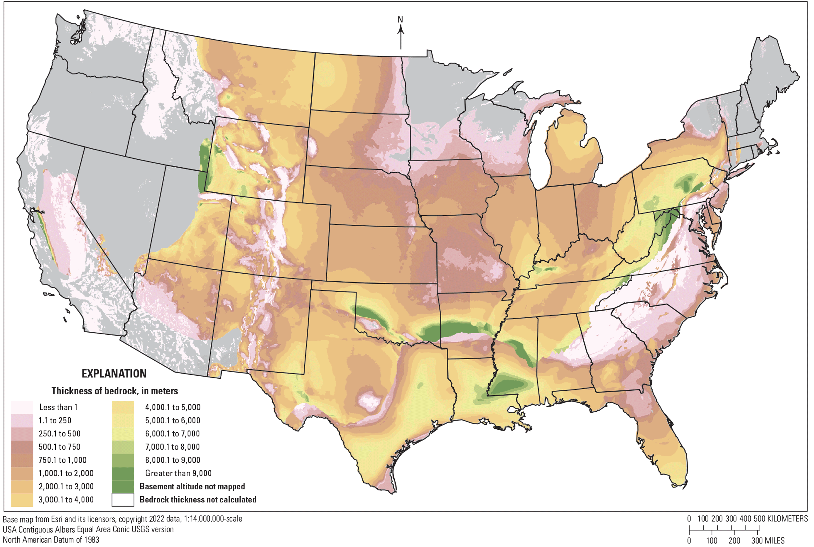
Map of the thickness of bedrock for the conterminous United States at a 2.5-kilometer resolution in the national three-layer geologic model. Below 1,000 meters, the color ramp includes intermediate intervals that highlight details of distribution of bedrock where it is relatively thin.
Discussion
The compilation of the top of bedrock and basement surfaces within the three-layer model cover a larger spatial extent and incorporate more data than almost any other GIS-based data compilations of national elevation surfaces. The compilation of the altitude of the top of basement rocks expands the spatial footprint of previous basement rock compilations (Domrois, 2013; Marshak and others, 2017a) by widening the definition of what is considered basement. In doing so, the digital compilation of the altitude of basement rocks becomes similar to previously published national-scale tectonic maps (Basement Rock Project Committee, 1967; Bayley and Muehlberger, 1968) and a national-scale map of total sediment thickness (Frezon and others, 1983). By extending the basement definition, the model expands its utility to all applications that may require an overall estimate of sediment thickness or depth to the crystalline rocks beneath sedimentary cover. Such uses might include deep aquifer and brackish water studies, depth estimates for assessments of deep geothermal energy potential and energy storage, estimates for assessment of certain critical minerals, or providing a generalization of crustal structure for ground shaking estimates and assessment of seismic hazard. The ability to look at elevation of specific geologic interfaces at the national scale provides a starting point for regional investigation of evolution and tectonic setting of sedimentary basins. The tabulation of unconsolidated deposits and sedimentary rocks that overlie bedrock allows for the depiction of young deposits and rocks that are omitted from some national-scale geologic maps (King and Beikman, 1974; Schruben and others, 1998; Garrity and Soller, 2009; Horton and others, 201764).
The 2.5-km cell dimensions within the national three-layer model were chosen primarily out of convenience to minimize computation time and screen refresh rates when working with the model in a GIS on a workstation computer. However, the limits of the scale of the 2.5-km cells, the national-scale model still faithfully captures the geometry of input datasets from both contoured data (Wyoming State Geological Survey, 2022; University of Nebraska–Lincoln, 2025141) and DEM-type gridded data (Illinois State Geological Survey, 2015). The cell-based compilation method also allows for side-by-side viewing of subsurface datasets to integrate adjacent individual maps, such as basement maps of Colorado (Hemborg, 1996) and Wyoming (Wyoming State Geological Survey, 2022).
The cell-based compilation method is modular and extensible, allowing for the incorporation of multiple topical studies and the ready revision of the bedrock or basement surface beyond the data currently (2025) compiled. In this way, the model can become part of the digital infrastructure of the USGS National Cooperative Geologic Mapping Program (NCGMP), providing the ability to ingest subsurface mapping and modeling products into a dynamic dataset as they are completed and submitted to the NCGMP.
The geocellular approach allows for elevation values and other attributes to be manually entered into the cell structure. The use of a GIS-based method facilitates the incorporation of geologic map data through the direct sampling of digital map data to cells at land surface. Within a 3-D modeling program, it is often tedious and difficult to match surface exposures directly because of the need to add abundant control points to adjust the shape of a grid to match mapped outcrop patterns. The GIS methodology allows direct manual editing of specific nodes, aiding, for example, the direct insertion of the amount of fault offset as a difference in elevation of adjacent cells.
The geocellular approach makes the use and editing of the model more accessible because users do not need to work in a 3-D geologic modeling program; most of the work can be done within a GIS. The resultant model file is compact because the GIS vector file is a “flattened” version of a volumetric model as a 2-D polygonal array of cells (and cell centroids) that are attributed with multiple z attribute values that represent tops and thickness of geologic units. Three-dimensional geologic models are labor intensive to build; require expensive software and skilled personnel; and can be difficult to distribute to colleagues, cooperators, and stakeholders. Building a model using the 2.5-D nature of a GIS (x and y dimension plus multiple z attribute values) can make a geologic model more accessible to project geologists and stakeholders.
Increasingly, numerical hydrologic models use sophisticated 3-D geological frameworks as their geologic input into the numerical simulation. There are a variety of numerical modeling platforms and no specific standards for the structuring of 3-D data; therefore, a simple, convenient method is needed to transfer geologic framework data to the numerical modeling software. The vector-based cell structure such as used by the three-layer model is readily transferable to process models such as finite difference models that use a cellular structure (Harbaugh, 2005). The geologic framework can be made to explicitly honor the x and y dimensions and cell size of the numerical hydrologic model and explicitly incorporate the numerical model’s DEM, easing the compatibility between geologic and numerical model.
Limitations of the Model and Method
Two types of limitations for this study can be identified: those related to the compilation method itself and those related to the data and decisions used to construct this specific model. The limitations of the overall methodology are difficult to address because they are inherently part of the model-building procedure. Limitations of this particular model could be addressed by using more data, developing a better data synthesis strategy, and creating more refined elevation surfaces to sample.
Limitations of the Compilation Method
One limitation of the three-layer model is that the compilation of the informal model units is dependent on the definition of each unit. Compilation using these informal units is useful in showing the overall shape and provides a consistent portrayal across broad areas with varied geology. However, the informal units are not readily combined with lithostratigraphically or chronostratigraphically defined units without a place-specific definitions list. Potential future national-scale compilations could be better served using chronostratigraphic units or with correlated lithostratigraphic units. Use of the informal subsurface mapping units across the Nation to provide spatial continuity creates a false equivalence between rock types and ages that obscures significant geologic and tectonic differences among regions.
The cell-based compilation method creates elevation surfaces in isolation as “flying carpets.” Reliance on a GIS does not take advantage of powerful aspects of 3-D geologic modeling software tools, such as using geologic rules like onlap and unconformities to control topology between different surfaces and volumes and generate realistic layering schemes. When values are assigned to every cell in the GIS-based approach, resultant grids may be over constrained, as compared to gridding from the input contour or well data. There is a limited ability to revise the elevation surfaces once values are assigned. If modifications are needed, individual cells must be edited manually.
Model construction using a cell-based compilation method is labor intensive, time consuming, and prone to errors. A model for the conterminous United States with cell dimensions of 2.5 km in x and y directions results in nearly 1.3 million cells, each of which has multiple attributes. Operating on this quantity of data manually allows for the possibility of introducing errors from the large amount of editing by hand and multiple manual steps needed to complete each surface. The edited surfaces tend to take on a ragged appearance with repeated manual edits and as the extent of datasets overlaps.
Limitations of This Model
The use of cell dimensions of 2.5 km in x and y directions constitutes a limitation of scale and resolution. Although cell dimensions could be modified and all input data could be resampled, the current 2.5-km grid cell size is useful when viewed at larger scales.
The present model was constructed without a defined procedure for how to incorporate new datasets and merge them into the existing dataset. Elevation data from separate studies were sampled with no regard to edge effects and no attempt at smoothing or checking for consistency with adjacent cells. At the scale of many kilometers, edge effects are not particularly noticeable but become apparent when zoomed in. During model construction, there was no defined evaluation process in place for reviewing datasets and making decisions about which dataset might be preferred in an area where several sources of data might be available. A general assumption was that newer, more current datasets would replace older ones, but the viability and practicality of this assumption was never tested.
The present three-layer model includes known omissions or inconsistencies that potentially could be addressed in a revised version of the model. Use of a grid defining the depth to Mesozoic basement for the Western United States (Shah and others, 2018) that was itself derived from national-scale sediment thickness map (Frezon and others, 1983) resulted in forcing the top of bedrock or base of Cenozoic rocks to the land surface in parts of the Pacific Northwest, where thick sections of Cenozoic volcanic rocks are mapped at land surface and are known to be many kilometers thick. In the Western United States, where subsurface data on the configuration of basement rocks are often lacking, igneous and metamorphic rock polygons were selected from digital geologic maps to augment the spatial extent of the basement layer. However, selection sets were dependent on the lithologic descriptors assigned to each polygon; these map-based selections could be improved with reference to more detailed geologic map data.
Summary
A digital three-layer geologic model of the conterminous United States has been constructed by mapping the altitude of three surfaces: land surface, the top of bedrock, and the top of basement. These surfaces are mapped through the compilation and synthesis of published stratigraphic horizons from numerous topical studies, but data compilation and synthesis were highly dependent on the definition of the informal terms “bedrock” and “basement.” Construction of a national-scale subsurface geologic model serves the needs of the U.S. Geological Survey as a fundamental starting point for national- to regional-scale resource assessments.
References Cited
Allmendinger, R.W., Hauge, T.A., Hauser, E.C., Potter, C.J., Klemperer, S.L., Nelson, K.D., Knuepfer, P., Oliver, J., 1987, Overview of the COCORP 40°N transect, Western United States—The fabric of an orogenic belt: Geological Society of America Bulletin, v. 98, no. 3, p. 308–319, accessed July 15, 2025, at https://doi.org/10.1130/0016-7606(1987)98%3C308:OOTCNT%3E2.0.CO;2.
Anderson, R.R., 1995, Map of configuration of Precambrian surface, Iowa, and surrounding areas: Iowa Geological and Water Survey Open File Map 95–2, scale 1:1,000,000, accessed August 24, 2023, at https://www.iihr.uiowa.edu/igs/publications/uploads/OFR-1995-2.pdf.
Arbenz, J.K., 2008, Structural framework of the Ouachita Mountains, in Suneson, N.H., ed., Stratigraphic and structural evolution of the Ouachita Mountains and Arkoma Basin, southeastern Oklahoma and west-central Arkansas—Applications to petroleum exploration—2004 field symposium: Oklahoma Geological Survey Circular 112A, p. 1–40, accessed July 16, 2025, at http://ogs.ou.edu/docs/circulars/C112A.pdf.
Association of American State Geologists, 2014, Resolution on AASG commitment to the role of geologic mapping in society: Association of American State Geologists Fact Sheet, 1 p., accessed March 6, 2023, at https://www.stategeologists.org/factsheets. [Fact sheet available using the “Lexington resolution on geologic mapping (2019-02-07)” link.]
Baars, D.L., Bartleson, B.L., Chapin, C.E., Curtis, B.F., De Voto, R.H., Everett, J.R., Johnson, R.C., Molenaar, C.M., Peterson, F., Schenk, C.J., Love, J.D., Merlin, I.S., Rose, P.R., Ryder, R.T., Waechter, N.B., and Woodward, L.A., 1988, Basins of the Rocky Mountain region, chap. 8 of Sloss, L.L., ed., Sedimentary cover—North American craton—U.S., v. D–2 of The geology of North America: Boulder, Colo., Geological Society of America, p. 109–220. [Also available at https://doi.org/10.1130/DNAG-GNA-D2.]
Baranoski, M.T., 2013, Structure contour map on the Precambrian unconformity surface in Ohio and related basement features (ver. 2.0): Ohio Department of Natural Resources, Division of Geological Survey Map PG–23, 17 p., 1 pl., scale 1:500,000, accessed August 24, 2024, at https://ohiodnr.gov/static/documents/geology/MapPG23_Baranoski_2013_text.pdf.
Basement Rock Project Committee, 1967, Basement map of North America between latitudes 24° and 60° N: Washington, D.C., American Association of Petroleum Geologists and U.S. Geological Survey, scale 1:5,000,000, accessed April 22, 2020, at https://www.loc.gov/resource/g3301c.ct003142/.
Battelle, 2005, The Midwest Regional Carbon Sequestration Partnership (MRCSP)—Phase 1 final report: U.S. Department of Energy, prepared by Battelle, under cooperative agreement no. DE-FC26-03NT41981, 284 p., accessed October 10, 2024, at https://doi.org/10.2172/889494.
Bayley, R.W., and Muehlberger, W.R., 1968, Basement rock map of the United States, exclusive of Alaska and Hawaii: U.S. Geological Survey, scale 1:2,500,000, accessed June 15, 2023, at https://doi.org/10.3133/70211241.
Belitz, K., Watson, E., Johnson, T.D., and Sharpe, J., 2019, Secondary hydrogeologic regions of the conterminous United States: Groundwater, v. 57, no. 3, p. 367–377, accessed August 31, 2023, at https://doi.org/10.1111/gwat.12806.
Bennett, V.C., and DePaolo, D.J., 1987, Proterozoic crustal history of the Western United States as determined by neodymium isotopic mapping: Geologic Society of America Bulletin, v. 99, no. 5, p. 674–685, accessed July 15, 2025, at https://pubs.geoscienceworld.org/gsa/gsabulletin/article-abstract/99/5/674/203256/Proterozoic-crustal-history-of-the-western-United.
Best, M.G., Christiansen, E.H., de Silva, S., and Lipman, P.W., 2016, Slab-rollback ignimbrite flareups in the southern Great Basin and other Cenozoic American arcs—A distinct style of arc volcanism: Geosphere, v. 12, no. 4, p. 1097–1135, accessed January 30, 2025, at https://doi.org/10.1130/GES01285.1.
Blakely, R.J., Jachens, R.C., Calzia, J.P., and Langenheim, V.E., 1999, Cenozoic basins of the Death Valley extended terrane as reflected in regional-scale gravity anomalies, in Wright, L.A., and Troxel, B.W., eds., Cenozoic basins of the Death Valley region: Boulder, Colo., Geological Society of America Special Paper 333, p. 1–16. [Also available at https://doi.org/10.1130/SPE333.]
Blakely, R.J., Morin, R.L., McKee, E.H., Schmidt, K.M., Langenheim, V.E., and Dixon, G.L., 1998, Three-dimensional model of Paleozoic basement beneath Amargosa Desert and Pahrump Valley, California and Nevada—Implications for tectonic evolution and water resources: U.S. Geological Survey Open-File Report 98–496, 29 p., accessed September 7, 2023, at https://doi.org/10.3133/ofr98496.
Blakely, R.J., and Ponce, D.A., 2001, Map showing depth to pre-Cenozoic basement in the Death Valley ground-water model area, Nevada and California: U.S. Geological Survey Miscellaneous Field Studies Map MF–2381–E, 1 sheet, scale 1:250,000, 6-p. pamphlet, accessed August 20, 2023, at https://doi.org/10.3133/mf2381E.
Boyd, O.S., 2019, 3D geologic framework for use with the U.S. Geological Survey National Crustal Model, phase 1—Western United States: U.S. Geological Survey Open-File Report 2019–1081, 36 p., accessed January 31, 2020, at https://doi.org/10.3133/ofr20191081.
Boyd, O.S., and Sweetkind, D.S., 2025, A comprehensive geologic framework of the National Crustal Model for seismic hazard studies in the conterminous United States: Lithosphere, no. 4, 16 p., accessed Jan 12, 2026 at https://doi.org/10.2113/2025/lithosphere_2025_117.
Bristol, R.S., Euliss, N.H., Jr., Booth, N.L., Burkardt, N., Diffendorfer, J.E., Gesch, D.B., McCallum, B.E., Miller, D.M., Morman, S.A., Poore, B.S., Signell, R.P., and Viger, R.J., 2013, U.S. Geological Survey core science systems strategy—Characterizing, synthesizing, and understanding the critical zone through a modular science framework: U.S. Geological Survey Circular 1383–B, 33 p. [Also available at https://doi.org/10.3133/cir1383B.]
Broadhead, R.F., Mansell, M., and Jones, G., 2009, Carbon dioxide in New Mexico—Geologic distribution of natural occurrences: New Mexico Bureau of Geology and Mineral Resources Open-File Report 514, 131 p., 3 appendixes and digital data, accessed July 7, 2023, at https://geoinfo.nmt.edu/publications/openfile/details.cfml?Volume=514.
Brock, J., Berry, K., Faulds, J., Berg, R., House, K., Marketti, M., McPhee, D., Schmidt, K., Schmitt, J., Soller, D., Spears, D., Thompson, R., Thorleifson, H., and Walsh, G., 2021, Renewing the National Cooperative Geologic Mapping Program as the Nation’s authoritative source for modern geologic knowledge: U.S. Geological Survey Open-File Report 2021–1013, 10 p., accessed May 12, 2021, at https://doi.org/10.3133/ofr20211013.
Bureau of Economic Geology, 2009, Integrated synthesis of the Permian Basin—Data and models for recovering existing and undiscovered oil resources from the largest oil-bearing basin in the U.S.: U.S. Department of Energy, prepared by Bureau of Economic Geology, University of Texas at Austin, under contract no. DE-FC26-04NT15509, 964 p., accessed June 2, 2020, at https://www.beg.utexas.edu/research/areas/permian-basin-synthesis.
Burgess, P.M., 2019, Phanerozoic evolution of the sedimentary cover of the North American craton, in Miall, A.D., ed., The sedimentary basins of the United States and Canada, v. 5 of Sedimentary basins of the world: Amsterdam, Netherlands, Elsevier, p. 31–63, accessed September 5, 2020, at https://doi.org/10.1016/B978-0-444-63895-3.00002-4.
Burns, E.R., Morgan, D.S., Peavler, R.S., and Kahle, S.C., 2011, Three-dimensional model of the geologic framework for the Columbia Plateau Regional Aquifer System, Idaho, Oregon, and Washington: U.S. Geological Survey Scientific Investigations Report 2010–5246, 44 p., accessed August 20, 2023, at https://pubs.usgs.gov/sir/2010/5246.
Campbell, B.G., and Coes, A.L., eds., 2010, Groundwater availability in the Atlantic Coastal Plain of North and South Carolina: U.S. Geological Survey Professional Paper 1773, 241 p., 7 pls., accessed September 28, 2020, at https://pubs.usgs.gov/pp/1773/.
Cannon, D.M., Bellino, J.C., and Williams, L.J., 2012, Digital surfaces and hydrogeologic data for the Mesozoic through early Tertiary rocks in the Southeastern Coastal Plain in parts of Mississippi, Alabama, Georgia, South Carolina, and Florida: U.S. Geological Survey Data Series 662, 13 p., with digital data, accessed August 27, 2023, at https://pubs.usgs.gov/ds/662/.
Cather, S.M., 2004, Laramide orogeny in central and northern New Mexico and southern Colorado, in Mack, G.H., and Giles, K.A., eds., The geology of New Mexico—A geologic history: New Mexico Geological Society, Special Publication 11, p. 203–248. [Also available at https://doi.org/10.56577/SP-11.]
Cederberg, J.R., Sweetkind, D.S., Buto, S.G., and Masbruch, M.D., 2011, Appendix 1—Three-dimensional hydrogeologic framework, in Heilweil, V.M., and Brooks, L.E., eds., Conceptual model of the Great Basin carbonate and alluvial aquifer system: U.S. Geological Survey Scientific Investigations Report 2010–5193, p. 127–141, accessed August 21, 2023, at https://doi.org/10.3133/sir20105193.
Cederstrand, J.R., and Becker, M.F., 1998, Digital map of base of aquifer for High Plains Aquifer in parts of Colorado, Kansas, Nebraska, New Mexico, Oklahoma, South Dakota, Texas, and Wyoming (1st ed.): U.S. Geological Survey Open-File Report 98–393, 1 computer diskette, accessed March 1, 2020, at https://doi.org/10.3133/ofr98393.
Cohee, G.V., 1962. Tectonic map of the United States, exclusive of Alaska and Hawaii: U.S. Geological Survey, scale 1:2,500,000, accessed August 31, 2023, at https://doi.org/10.3133/70211240.
Cole, V.B., 1976, Configuration of the top of Precambrian rocks in Kansas: Kansas Geological Survey, Map M–7, scale 1:500,000, accessed August 24, 2023, at https://www.kgs.ku.edu/Publications/Bulletins/Map7/ks_precambrian_map.pdf.
Coleman, J.L., Jr., and Cahan, S.M., 2012, Preliminary catalog of the sedimentary basins of the United States: U.S. Geological Survey Open-File Report 2012–1111, 27 p., accessed August 7, 2021, at https://doi.org/10.3133/ofr20121111. [Four figures and one table available as separate files.]
Colgan, J.P., Egger, A.E., John, D.A., Cousens, B., Fleck, R.J., and Henry, C.D., 2011, Oligocene and Miocene arc volcanism in northeastern California—Evidence for post-Eocene segmentation of the subducting Farallon plate: Geosphere, v. 7, no. 3, p. 733–755, accessed August 21, 2023, at https://doi.org/10.1130/GES00650.1.
Consortium for Spatial Information, 2018, SRTM 90m DEM digital elevation database (ver. 4, November 2018): Consortium for Spatial Information, accessed March 20, 2020, at http://srtm.csi.cgiar.org.
Crain, K.D., and Chang, J.C., 2018, Elevation map of the top of the crystalline basement in Oklahoma and surrounding States: Oklahoma Geological Survey Open-File Report 1–2018, 6 p., accessed September 6, 2023, at https://www.ou.edu/ogs/publications/openfilereports. [Separately downloadable digital GIS data file “Open-File Report 1–2018 Supplement” also available.]
Csontos, R., and Van Arsdale, R., 2008, New Madrid seismic zone fault geometry: Geosphere, v. 4, no. 5, p. 802–813, accessed October 10, 2024, at https://doi.org/10.1130/GES00141.1.
Dechesne, M., Raynolds, R.G., Barkmann, P.E., and Johnson, K.R., 2011, Notes on the Denver Basin geologic maps—Bedrock geology, structure, and isopach maps of the Upper Cretaceous to Paleogene Strata between Greeley and Colorado Springs, Colorado: Colorado Geological Survey OF–11–01, 35 p., 13 pl., plus digital database, accessed June 15, 2023, at https://coloradogeologicalsurvey.org/publications/geologic-map-stratigraphy-notes-denver-basin-colorado/.
Dickinson, W.R., Klute, M.A., Hayes, M.J., Janecke, S.U., Lundin, E.R., McKittrick, M.A., and Olivares, M.D., 1988, Paleogeographic and paleotectonic setting of Laramide sedimentary basins in the central Rocky Mountain region: Geological Society of America Bulletin, v. 100, no. 7, p. 1023–1039, accessed May 15, 2023, at https://doi.org/10.1130/0016-7606(1988)100%3C1023:PAPSOL%3E2.3.CO;2.
Dixon, J.S., 1982, Regional structural synthesis, Wyoming salient of western overthrust belt: American Association of Petroleum Geologists Bulletin, v. 66, no. 10, p. 1560–1580, accessed August 22, 2023, at https://doi.org/10.1306/03b5a98a-16d1-11d7-8645000102c1865d.
Domrois, S.L., 2013, The Midcontinent exposed—Precambrian basement topography, and fault-and-fold zones, within the cratonic platform of the United States: Urbana, Illinois, University of Illinois at Urbana–Champaign, M.S. thesis, 90 p., accessed August 22, 2023, at https://www.ideals.illinois.edu/items/45519.
Ewing, T.E., Barnes, M.A., and Denison, R.E., 2019, Proterozoic foundations of the Permian Basin, West Texas and southeastern New Mexico—A review, chap. 3 of Ruppel, S.C., ed., Anatomy of a Paleozoic basin—The Permian Basin, USA [v. 1]: University of Texas at Austin, Bureau of Economic Geology Report of Investigations 285, American Association of Petroleum Geologists Memoir 118, p. 43–61. [Also available at https://doi.org/10.23867/RI0285-1.]
Faunt, C.C., 2006, Surface altitudes of hydrogeologic units used in the hydrogeologic framework and transient ground-water flow model of the Death Valley regional ground-water flow system, Nevada and California: U.S. Geological Survey data release, accessed September 30, 2023, at https://doi.org/10.5066/P9176K3Z.
Faunt, C.C., Sweetkind, D.S., and Belcher, W.R., 2010, Hydrogeologic framework model, chap. E of Belcher, W.R., and Sweetkind, D.S., eds., 2010, Death Valley regional ground-water flow system, Nevada and California—Hydrogeologic framework and transient ground-water flow model: U.S. Geological Survey Professional Paper 1711, p. 161–249, accessed August 22, 2023, at https://pubs.usgs.gov/pp/1711/.
Flawn, P.T., 1965, Basement—Not the bottom but the beginning: American Association of Petroleum Geologists Bulletin, v. 49, no. 7, p. 883−886, accessed September 18, 2023, at https://doi.org/10.1306/A663367A-16C0-11D7-8645000102C1865D.
Florio, G., 2020, The estimation of depth to basement under sedimentary basins from gravity data—Review of approaches and the ITRESC method, with an application to the Yucca Flat Basin (Nevada): Surveys in Geophysics, v. 41, p. 935–961, accessed September 7, 2023, at https://doi.org/10.1007/s10712-020-09601-9.
Frezon, S.I., Finn, T.M., and Lister, J.H., comps., 1983, Total thickness of sedimentary rocks in the conterminous United States: U.S. Geological Survey Open-File Report 83–920, 1 pl. [Also available at https://doi.org/10.3133/ofr83920.]
Garrity, C.P., and Soller, D.R., 2009, Database of the geologic map of North America—Adapted from the map by J.C. Reed, Jr. and others (2005): U.S. Geological Survey Data Series 424, accessed February 2, 2025, at https://doi.org/10.3133/ds424.
Gelman, S.E., and Johnson, B.G., 2023, Data release for the 3D petroleum systems model of the Williston Basin, USA: U.S. Geological Survey data release, accessed August 22, 2023, at https://doi.org/10.5066/P9N7O1OT.
Gill, J.R., and Cobban, W.A., 1973, Stratigraphy and geologic history of Montana Group and equivalent rocks, Montana, Wyoming, and North and South Dakota: U.S. Geological Survey Professional Paper, 776, 37 p., accessed August 16, 2023, at https://doi.org/10.3133/pp776.
Goldberg, J., 2025, Digital database of a 3D geological model of the Denver Basin: U.S. Geological Survey data release, accessed July 9, 2025, at https://doi.org/10.5066/P14PSVBV.
Grauch, V.J.S., Rodriquez, B.D., and Wooden, J.L., 2003, Geophysical and isotopic constraints on crustal structure related to mineral trends in north-central Nevada and implications for tectonic history: Economic Geology, v. 98, no. 2, p. 269–286, accessed July 15, 2025, at http://dx.doi.org/10.2113/gsecongeo.98.2.269.
Gundersen, L.C.S., Belnap, J., Goldhaber, M., Goldstein, A., Haeussler, P.J., Ingebritsen, S.E., Jones, J.W., Plumlee, G.S., Thieler, E.R., Thompson, R.S., and Back, J.M., 2011, Geology for a changing world 2010–2020—Implementing the U.S. Geological Survey science strategy: U.S. Geological Survey Circular 1369, 68 p., accessed March 6, 2023, at https://pubs.usgs.gov/circ/circ1369/.
Gutentag, E.D., Heimes, F.J., Krothe, N.C., Luckey, R.R., and Weeks, J.B., 1984, Geohydrology of the High Plains Aquifer in parts of Colorado, Kansas, Nebraska, New Mexico, Oklahoma, South Dakota, Texas, and Wyoming: U.S. Geological Survey Professional Paper 1400–B, 63 p., accessed March 1, 2020, at https://doi.org/10.3133/pp1400B.
Harbaugh, A.W., 2005, MODFLOW-2005, The U.S. Geological Survey modular ground-water model—The ground-water flow process: U.S. Geological Survey Techniques and Methods 6–A16, book 16, chap. A16, [variously paged], accessed February 25, 2025, at https://pubs.usgs.gov/tm/2005/tm6A16/PDF/TM6A16.pdf.
Hart, D.J., Mauel, S.W., Luczaj, J.A., and Stewart, E.K., 2021, Depth-to-bedrock mapping in Wisconsin: Wisconsin Geological and Natural History Survey Open-File Report 2021–04, 46 p., accessed September 7, 2023, at https://wgnhs.wisc.edu/catalog/publication/000982/resource/wofr202104.
Harwood, D.S., and Helley, E.J., 1987, Late Cenozoic tectonism of the Sacramento Valley, California: U.S. Geological Survey Professional Paper 1359, 46 p., 1 pl., scale 1:250,000. [Also available at https://doi.org/10.3133/pp1359.]
Hatcher, R.D., Jr., 1989, Tectonic synthesis of the U.S. Appalachians, in Hatcher, R.D., Jr., Thomas, W.A., and Viele, G.W., eds., The Appalachian-Ouachita Orogen in the United States: Boulder, Colo., Geological Society of America, The Geology of North America, v. F–2, p. 511–535. [Also available at https://doi.org/10.1130/DNAG-GNA-F2.511.]
Hatcher, R.D., Jr., Lemiszki, P.J., and Whisner, J.B., 2007, Character of rigid boundaries and internal deformation of the southern Appalachian foreland fold-thrust belt, in Sears, J.W., Harms, T.A., and Evenchick, C.A., eds., Whence the mountains? Inquiries into the evolution of orogenic systems—A volume in honor of Raymond A. Price: Geological Society of America Special Paper no. 433, p. 243–276, accessed August 15, 2021, at https://doi.org/10.1130/2007.2433(12).
Heffner, D.M., 2013, Tectonics of the South Georgia Rift: Columbia, S.C., University of South Carolina, Ph.D. dissertation, 177 p., accessed June 12, 2023, at https://scholarcommons.sc.edu/etd/1330.
Hemborg, H.T., 1996, MS-30 basement structure map of Colorado with major oil and gas fields: Colorado Geological Survey Department of Natural Resources Map Series no. 30, 1 p., scale 1:1,000,000, accessed August 24, 2023, at https://doi.org/10.58783/cgs.ms30.lpgm7980.
Herrick, S.M., and Vorhis, R.C., 1963, Subsurface geology of the Georgia Coastal Plain: Georgia Geologic Survey Information Circular 25, 78 p., accessed September 28, 2020, at https://epd.georgia.gov/document/publication/ic-25-subsurface-geology-georgia-coastal-plain-1963/download.
Herzog, B.L., Stiff, B.J., Chenoweth, C.A., Warner, K.L., Sievering, J.B., and Avery, C., 1994, Buried bedrock surface of Illinois: Illinois State Geological Survey Map Series, Illinois Map 5, scale 1:500,000, accessed August 31, 2023, at https://resources.isgs.illinois.edu/maps/buried-bedrock-surface-illinois.
Hills, J.M., 1984, Sedimentation, tectonism, and hydrocarbon generation in Delaware Basin, west Texas and southeastern New Mexico: AAPG Bulletin, v. 68, p. 250–267, accessed August 22, 2023, at https://doi.org/10.1306/ad460a08-16f7-11d7-8645000102c1865d.
Horton, J.D., San Juan, C.A., and Stoeser, D.B., 2017, The State Geologic Map Compilation (SGMC) geodatabase of the conterminous United States (ver. 1.1, August 2017): U.S. Geological Survey Data Series 1052, 46 p., accessed April 2, 2020, at https://doi.org/10.3133/ds1052.
Hosman, R.L., 1996, Regional stratigraphy and subsurface geology of Cenozoic deposits, Gulf Coastal Plain, South-Central United States: U.S. Geological Survey Professional Paper 1416–G, 35 p., 14 pl., accessed April 10, 2020, at https://doi.org/10.3133/pp1416G.
Illinois State Geological Survey, 2015, Geologic and geophysical maps of the Ozark, Illinois, Indiana, and Kentucky (OIINK) region: Illinois State Geological Survey Geospatial Data Clearinghouse, accessed May 24, 2020, at http://clearinghouse.isgs.illinois.edu/data/geology/geologic-and-geophysical-maps-ozark-illinois-indiana-and-kentucky-oiink-region.
Jachens, R.C., and Moring, B.C., 1990, Maps of the thickness of Cenozoic deposits and the isostatic residual gravity over basement for Nevada: U.S. Geological Survey Open-File Report 90–404, 15 p., accessed August 20, 2023, at https://doi.org/10.3133/ofr90404.
Johnson, R.C., Mercier, T.J., and Brownfield, M.E., 2011, Assessment of in-place oil shale resources of the Green River Formation, Greater Green River Basin in Wyoming, Colorado, and Utah: U.S. Geological Survey Fact Sheet 2011–3063, 4 p., accessed January 27, 2026, at https://doi.org/10.3133/fs20113063.
Johnson, R.C., and Roberts, S.B., 2003, The Mesaverde total petroleum system, Uinta-Piceance Province, Utah and Colorado, chap. 7 of Petroleum systems and geologic assessment of oil and gas in the Uinta-Piceance Province, Utah and Colorado: U.S. Geological Survey Digital Data Series DDS–69–B, 68 p., accessed June 20, 2020, at https://doi.org/10.3133/ds69B.
Khatiwada, M., and Keller, G.R., 2015, An integrated geophysical imaging of the upper-crustal features in the Harney Basin, southeast Oregon: Geosphere, v. 11, no. 1, p. 185–200, accessed August 21, 2023, at https://doi.org/10.1130/GES01046.1.
King, P.B., 1969, Tectonic map of North America: U.S. Geological Survey, scale 1:5,000,000, accessed April 15, 2020, at https://doi.org/10.3133/70211238.
King, P.B., and Beikman, H.M., 1974, Geologic map of the United States (exclusive of Alaska and Hawaii): U.S. Geological Survey, scale 1:2,500,000, 2 pl. [Also available at https://pubs.usgs.gov/publication/70136641.]
Langenheim, V.E., Glen, J.M., Jachens, R.C., Dixon, G.L., Katzer, T.C., and Morin, R.L., 2000, Geophysical constraints on the Virgin River Depression, Nevada, Utah, and Arizona: U.S. Geological Survey Open-File Report 00–407, 28 p., accessed September 7, 2023, at https://pubs.usgs.gov/of/2000/0407/.
Larsen, J.H., 1983, Hanna, Laramie and Shirley Basins: Earth Science Bulletin, v. 16, no. 1, p. 23–62, accessed January 30, 2025, at https://archives-datapages-com.usgslibrary.idm.oclc.org/data/wyoming-geo-assoc-earth-science-bull/data/016/016001/pdfs/23.pdf.
Lawrence, D.P., and Hoffman, C.W., 1993, Geology of basement rocks beneath the North Carolina Coastal Plain: North Carolina Geological Survey Bulletin 95, 60 p., 1 pl., accessed September 4, 2023, at https://digital.ncdcr.gov/Documents/Detail/geology-of-basement-rocks-beneath-the-north-carolina-coastal-plain/3691954.
Lawton, T.F., 2008, Laramide Sedimentary Basins, chap. 8 of Miall, A.D., ed., The sedimentary basins of the United States and Canada, v. 5 of Sedimentary basins of the world: Netherlands, Elsevier, p. 429–450, accessed July 11, 2023, at https://doi.org/10.1016/S1874-5997(08)00012-9.
Levy, M., and Christie-Blick, N., 1989, Pre-Mesozoic palinspastic reconstruction of the eastern Great Basin (Western United States): Science, v. 245, no. 4925, p. 1454–1462, accessed July 15, 2025, at https://doi.org/10.1126/science.245.4925.1454.
Love, J.D., Christiansen, A.C., and Ver Ploeg, A.J., comps., 1993, Stratigraphic chart showing Phanerozoic nomenclature for the State of Wyoming: Geological Survey of Wyoming [Wyoming State Geological Survey] Map Series MS–41, 1 pl., accessed January 30, 2025, at https://sales.wsgs.wyo.gov/stratigraphic-chart-showing-phanerozoic-nomenclature-for-the-state-of-wyoming-1993/.
Lund, K., Box, S.E., Holm-Denoma, C.S., San Juan, C.A., Blakely, R.J., Saltus, R.W., Anderson, E.D., and DeWitt, E.H., 2015, Basement domain map of the conterminous United States and Alaska: U.S. Geological Survey Data Series 898, 41 p., accessed August 25, 2023, at https://doi.org/10.3133/ds898.
Lynds, R.M., and Carroll, C.J., 2015, Stratigraphic cross sections and subsurface model of the Lance and Fort Union formations, Great Divide Basin, Wyoming: Wyoming State Geological Survey Open-File Report 15–3, 1 pl., accessed June 30, 2020, at https://sales.wsgs.wyo.gov/stratigraphic-cross-sections-and-subsurface-model-of-the-lance-and-fort-union-formations-great-divide-basin-wyoming-2015/.
Macfarlane, P.A., and Wilson, B.B., 2019, Enhancement of the bedrock-surface-elevation map beneath the Ogallala portion of the High Plains Aquifer, western Kansas: Kansas Geological Survey Technical Series 20, 34 p., 2 pl., accessed September 7, 2023, at https://www.kgs.ku.edu/Publications/Bulletins/TS20/index.html#PLATES.
Mankinen, E.A., Hildenbrand, T.G., Zientek, M.L., Box, S.E., Bookstrom, A.A., Carlson, M.H., and Larsen, J.C., 2004, Guide to geophysical data for the northern Rocky Mountains and adjacent areas, Idaho, Montana, Washington, Oregon, and Wyoming (ver. 1.1, October 2, 2005): U.S. Geological Survey Open-File Report 2004–1413, 34 p. with digital data, accessed August 20, 2023, at https://pubs.usgs.gov/of/2004/1413/.
Manspeizer, W., DeBoer, J., Costain, J.K., Froelich, A.J., Çoruh, C., Olsen, P.E., McHone, G.J., Puffer, J.H., and Prowell, D.C., 1989, Post-Paleozoic activity, in Hatcher, R.D., Jr., Thomas, W.A., and Viele, G.W., eds., The Appalachian-Ouachita Orogen in the United States: Boulder, Colo., Geological Society of America, v. F–2, p. 319–374. [Also available at https://doi.org/10.1130/DNAG-GNA-F2.319.]
Marshak, S., Domrois, S., Abert, C., and Larson, T., 2017a, Supplemental material—The basement revealed—Tectonic insight from a digital elevation model of the Great Unconformity, USA cratonic platform: The Geological Society of America Data Repository Item 2017115, accessed March 18, 2020, at https://doi.org/10.1130/2017115. [Alternative data location is served by University of Illinois at Urbana–Champaign at https://doi.org/10.13012/B2IDB-7546972_V1.]
Marshak, S., Domrois, S., Abert, C., Larson, T., Pavlis, G., Hamburger, M., Yang, X., Gilbert, H., and Chen, C., 2017b, The basement revealed—Tectonic insight from a digital elevation model of the Great Unconformity, USA cratonic platform: Geology, v. 45, no. 5, p. 391−394, accessed May 24, 2020, at https://doi.org/10.1130/G38875.1.
Martin, L.J., 1996, Geohydrology of tertiary rocks in the Green River structural basin in Wyoming, Utah, and Colorado: U.S. Geological Survey Water-Resources Investigations Report 92–4164, 43 p., accessed June 30, 2020, at https://doi.org/10.3133/wri924164.
McBride, J.H., Keach,R.,W., II, Leetaru, H.E., and Smith, K.M., 2018, Visualizing Precambrian basement tectonics beneath a carbon capture and storage site, Illinois Basin: Interpretation, v. 6, no. 2, p. T257–T270, accessed October 10, 2024, at https://doi.org/10.1190/INT-2017-0116.1.
McFarland, E.R., and Bruce, T.S., 2006, The Virginia Coastal Plain hydrogeologic framework: U.S. Geological Survey Professional Paper 1731, 118 p., 25 pls., accessed August 20, 2023, at https://doi.org/10.3133/pp1731.
Mills, S.A., Boyd, O.S., and Rukstales, K.S., 2020, Digitized datasets of the structure of Cenozoic and late Cretaceous strata along the Atlantic and Gulf Coastal Plains from Texas to New Jersey: U.S. Geological Survey data release, accessed September 28, 2020, at https://doi.org/10.5066/P9YXMZMJ.
Muehlberger, W.R., comp., 1992, Tectonic map of North America: Tulsa, Okla., American Association of Petroleum Geologists, scale 1:5,000,000, accessed June 10, 2020, at https://www.datapages.com/gis-map-publishing-program/subscription-content-downloadable-files-groups/north-central-america. [Link is not active in 2026. AAPG is in the process of converting digital data site to a subscription service.]
Nebraska Oil and Gas Conservation Commission, 2025, RBDMS [WellFinder]: Nebraska Oil and Gas Conservation Commission, accessed May 2022 at http://www.nogcc.ne.gov/NOGCCOnlineGIS/.
Nebraska Water Science Center, 2016, Base of aquifer contours for the Northern High Plains aquifer: U.S. Geological Survey data release, accessed March 11, 2020, at https://doi.org/10.5066/F7K072C9.
Neuendorf, K.K.E., Mehl, J.P., Jr., and Jackson, J.A., eds., 2011, Glossary of geology (5th ed. revised): American Geosciences Institute, Alexandria, Va., 779 p., accessed September 18, 2023, at https://www.americangeosciences.org/pubs/glossary.
Ohio Division of Geological Survey, 2003, Shaded bedrock-topography map of Ohio: Ohio Department of Natural Resources Division of Geological Survey Map BG–3, scale 1:2,000,000, accessed August 31, 2023, at https://ohiodnr.gov/static/documents/geology/MiscMap_OhioShadedBedrockTopography_2003.pdf.
Olsen, B.M., and Mossler, J.H., 1982, S–14 geologic map of Minnesota, depth to bedrock: University of Minnesota Digital Conservancy Minnesota Geological Survey State Map Series S–14, scale 1:1,000,000, accessed August 31, 2023, at https://hdl.handle.net/11299/60080.
Parker, S.E., 1986, Structure contour map on top of the uppermost Cretaceous Lance Formation, Bighorn Basin, Wyoming: Wyoming State Geological Survey Open File Report 86–6, 1 sheet, accessed June 15, 2020, at https://sales.wsgs.wyo.gov/structure-contour-map-on-top-of-the-uppermost-cretaceous-lance-formation-bighorn-basin-wyoming-1986/.
Pelletier, J.D., Broxton, P.D., Hazenberg, P., Zeng, X., Troch, P.A., Niu, G.-Y., Williams, Z., Brunke, M.A., and Gochis, D., 2016, A gridded global data set of soil, intact regolith, and sedimentary deposit thicknesses for regional and global land surface modeling: Journal of Advances in Modeling Earth Systems, v. 8, no. 1, p. 41–65, accessed January 30, 2025, at https://doi.org/10.1002/2015MS000526.
Ponce, D.A., and Glen, J.M.G., 2008, A prominent geophysical feature along the northern Nevada rift and its geologic implications, north-central Nevada: Geosphere, v. 4, no. 1, p. 207–217, accessed August 20, 2023, at https://doi.org/10.1130/GES00117.1.
Poole, F.G., Perry, W.J., Jr., Madrid, R.J., and Amaya-Martínez, R., 2005, Tectonic synthesis of the Ouachita-Marathon-Sonora orogenic margin of southern Laurentia—Stratigraphic and structural implications for timing of deformational events and plate-tectonic model, in Anderson, T.H., Nourse, J.A., McKee, J.W., and Steiner, M.B., eds., The Mojave-Sonora megashear hypothesis—Development, assessment, and alternatives: Geological Society of America Special Paper 393, p. 543–596, accessed August 25, 2023, at https://doi.org/10.1130/0-8137-2393-0.543.
Pope, J.P., Andreasen, D.C., McFarland, E.R., and Watt, M.K., 2016, Digital elevations and extents of regional hydrogeologic units in the Northern Atlantic Coastal Plain aquifer system from Long Island, New York, to North Carolina: U.S. Geological Survey Data Series 996, 28 p., accessed September 28, 2020, at https://doi.org/10.3133/ds996.
Powars, D.S., Johnson, G.H., Edwards, L.E., and Berquist, C.R., 2014, Geology of the Virginia Coastal Plain—New insights from continuous cores and geophysical surveys, in Bailey, C.M., Sherwood, W.C., Eaton, L.S., and Powars, D.S., eds., Geology of Virginia: Virginia Museum of Natural History Special Publication no. 18, p. 109–159, accessed September 28, 2020, at https://www.vmnh.net/research-collections/vmnh-scientific-publications/special-publications.
Reed, J.C., Jr., Bickford, M.E., Houston, R.S., Link, P.K., Rankin, D.W., Sims, P.K., and Van Schmus, W.R., eds., 1993, Precambrian—Conterminous U.S.: Boulder, Colo., Geological Society of America, The Geology of North America, v. C–2, 657 p., accessed August 31, 2023, at https://doi.org/10.1130/DNAG-GNA-C2.
Renken, R.A., 1996, Hydrogeology of the Southeastern Coastal Plain aquifer system in Mississippi, Alabama, Georgia, and South Carolina: U.S. Geological Survey Professional Paper 1410–B, 101 p., 42 pls., accessed August 24, 2023, at https://doi.org/10.3133/pp1410B.
Richard, S.M., Shipman, T.C., Greene, L.C., and Harris, R.C., 2007, Estimated depth to bedrock in Arizona, v. 1.0: Arizona Geological Survey Digital Geologic Map DGM–52, 1 pl., scale 1:1,000,000, 9 p., accessed September 7, 2023, at http://hdl.handle.net/10150/630081.
Roberts, S.B., Roberts, L.N.R., and Cook, T., 2007, Geologic assessment of undiscovered petroleum resources in the Waltman Shale Total Petroleum System, Wind River Basin Province, Wyoming, chap. 5 of Petroleum systems and geologic assessment of oil and gas in the Wind River Basin Province, Wyoming: U.S. Geological Survey Digital Data Series DDS–69–J, 32 p., accessed July 10, 2020, at https://doi.org/10.3133/ds69J.
Saltus, R.W., and Jachens, R.C., 1995, Gravity and basin-depth maps of the Basin and Range Province, Western United States: U.S. Geological Survey Geophysical Investigation Map GP–1012, 1 sheet, scale 1:2,500,000, accessed August 20, 2023, at https://doi.org/10.3133/gp1012.
Sawyer, D.S., Buffler, R.T., and Pilger, R.H., Jr., 1991, The crust under the Gulf of Mexico Basin, in Salvador, A., ed., The Gulf of Mexico Basin: Boulder, Colo., Geological Society of America, The Geology of North America, v. J, p. 53–72. [Also available at https://doi.org/10.1130/DNAG-GNA-J.53.]
Schlische, R.W., 1993, Anatomy and evolution of the Triassic–Jurassic Continental Rift System, eastern North America: Tectonics, v. 12, no. 4, p. 1026–1042, accessed June 12, 2023, at https://agupubs.onlinelibrary.wiley.com/doi/pdfdirect/10.1029/93TC01062.
Schruben, P.G., Arndt, R.E., and Bawiec, W.J., 1998, Geology of the conterminous United States at 1:2,500,000 scale—A digital representation of the 1974 P.B. King and H.M. Beikman map: U.S. Geological Survey Digital Data Series 11, release 2, accessed April 21, 2020, at https://pubs.usgs.gov/dds/dds11/.
Shah, A.K., and Boyd, O.S., 2018, Depth to basement and thickness of unconsolidated sediments for the Western United States— Initial estimates for layers of the U.S. Geological Survey National Crustal Model: U.S. Geological Survey Open-File Report 2018–1115, 13 p., accessed January 31, 2020, at https://doi.org/10.3133/ofr20181115.
Shah, A., Langenheim, V., and Boyd, O., 2018, Depth to Mesozoic basement for the Western United States—Data files of the U.S. Geological Survey National Crustal Model: U.S. Geological Survey data release, accessed January 31, 2020, at https://doi.org/10.5066/P9X5ZX6Y.
Shuster, M.W., Zahm, C.K., and Hennings, P.H., 2021, Oil and gas in fractured crystalline igneous and metamorphic rocks—Global overview and examples from Texas, chap. 3 of Callahan, O. A., and Eichhubl, P., eds., The geologic basement of Texas—A volume in honor of Peter T. Flawn: The University of Texas at Austin, Bureau of Economic Geology Report of Investigations no. 286, 70 p., accessed September 26, 2023, at https://doi.org/10.23867/RI0286C3.
Sims, P.K., 1990, Precambrian basement map of the northern midcontinent, U.S.A.: U.S. Geological Survey Miscellaneous Investigations Series Map I–1853–A, 1 sheet, scale 1:1,000,000, accessed September 4, 2023, at https://doi.org/10.3133/i1853A.
Sims, P.K., Peterman, Z.E., Hildenbrand, T.G., and Mahan, S., 1992, Precambrian basement map of the Trans-Hudson orogen and adjacent terranes, northern Great Plains, U.S.A.: U.S. Geological Survey Miscellaneous Investigations Series Map I–2214, 1 pl., scale 1:1,000,000, 56-p. pamphlet, accessed September 4, 2023, at https://doi.org/10.3133/i2214.
Sims, P.K., Saltus, R.W., and Anderson, E.D., 2008, Precambrian basement structure map of the continental United States—An interpretation of geologic and aeromagnetic data: U.S. Geological Survey Scientific Investigations Map 3012, scale 1:8,000,000, accessed September 4, 2023, at https://pubs.usgs.gov/sim/3012/.
Sloss, L.L., ed., 1988, Tectonic evolution of the craton in Phanerozoic time, in Sedimentary cover—North American craton: Boulder, Colo., Geological Society of America, Geology of North America, v. D–2, p. 25–52, accessed June 5, 2020, at https://doi.org/10.1130/DNAG-GNA-D2.
Snedden, J.W., and Galloway, W.E., 2019, The Gulf of Mexico sedimentary basin—Depositional evolution and petroleum applications: Cambridge, United Kingdom, Cambridge University Press, 326 p., https://doi.org/10.1017/9781108292795.
Soller, D.R., and Garrity, C.P., 2018, Quaternary sediment thickness and bedrock topography of the glaciated United States east of the Rocky Mountains: U.S. Geological Survey Scientific Investigations Map 3392, 2 sheets, scale 1:5,000,000, accessed January 2018 at https://doi.org/10.3133/sim3392.
Soller, D.R., Packard, P.H., and Garrity, C.P., 2012, Database for USGS Map I–1970—Map showing the thickness and character of Quaternary sediments in the glaciated United States east of the Rocky Mountains: U.S. Geological Survey Data Series 656, accessed April 21, 2020, at https://pubs.usgs.gov/ds/656/.
Soller, D.R., and Reheis, M.C., comps., 2004, Surficial materials in the conterminous United States: U.S. Geological Survey Open-file Report 03–275, scale 1:5,000,000, accessed April 21, 2020, at https://pubs.usgs.gov/of/2003/of03-275/.
Soller, D.R., Reheis, M.C., Garrity, C.P., and Van Sistine, D.R., 2009, Map database for surficial materials in the conterminous United States: U.S. Geological Survey Data Series 425, scale 1:5,000,000, accessed April 21, 2020, at https://pubs.usgs.gov/ds/425/.
Spangler, L.R., 2024a, Digital data for a 3D geological model of western South Dakota: U.S. Geological Survey data release, accessed July 9, 2025, at https://doi.org/10.5066/P9LK4QHJ.
Spangler, L.R., 2024b, Digital database of a 3D geological model of the Powder River Basin and Williston Basin regions, USA: U.S. Geological Survey data release, accessed September 21, 2024, at https://doi.org/10.5066/P13RSCBV.
Spangler, L., Melick, J., and Sweetkind, D., 2023, Digital subsurface database of elevation point data and structure contour maps of multiple subsurface units, Powder River Basin, Wyoming and Montana, USA: U.S. Geological Survey data release, accessed August 22, 2023, at https://doi.org/10.5066/P953MC5C.
Sweetkind, D.S., Cederberg, J.R., Buto, S.G., Masbruch, M.D., Smout, B., 2026, Digital input data and model output for a three-dimensional hydrogeologic framework for the Great Basin carbonate and alluvial aquifer system of Nevada, Utah, and parts of adjacent States: U.S. Geological Survey data release, accessed January 23, 2026, at https://doi.org/10.5066/P13BAFSV.
Sweetkind, D.S., Colgan, J.P., Smout, B., and Barrette, N.C., 2023a, Surface and subsurface geologic data from previous USGS studies of the Gulf Coast region, south-central United States: U.S. Geological Survey data release, accessed April 18, 2023, at https://doi.org/10.5066/P9F0X0YF.
Sweetkind, D.S., Dickerson, R.P., Blakely, R., and Denning, P.D., 2001, Interpretive geologic cross sections for the Death Valley regional flow system and surrounding areas, Nevada and California: U.S. Geological Survey Miscellaneous Field Studies Map MF–2370, 3 pls., 32-p. pamphlet. [Also available https://pubs.usgs.gov/mf/2001/mf-2370/.]
Sweetkind, D.S., Masbruch, M.D., Longley, P.C., Smout, B., and Goldberg, J., 2023b, Digital hydrogeologic framework model of the Upper Colorado River Basin, Western U.S.: U.S. Geological Survey data release, accessed August 1, 2023, at https://doi.org/10.5066/P96WFS3T.
Sweetkind, D.S., Zellman, K.L., and Goldberg, J., 2024, Preliminary digital data for a 3-layer geologic model of the conterminous United States using land surface, top of bedrock, and top of basement (ver. 1.1, April 2025): U.S. Geological Survey data release, accessed February 1, 2025, at https://doi.org/10.5066/P9LGSI6Q.
Swinehart, J.B., Souders, U.C., DeGraw, H.M., and Diffendal, R.F., Jr., 1985, Cenozoic paleogeography of Nebraska, in Flores, R.M., and Kaplan, S.S., eds., Cenozoic paleogeography of the west-central United States: Rocky Mountain Section Society of Economic Paleontologists and Mineralogists, p. 209–229, accessed August 13, 2023, at https://digitalcommons.unl.edu/diffendal/28.
Thamke, J.N., LeCain, G.D., Ryter, D.W., Sando, R., and Long, A.J., 2014, Hydrogeologic framework of the uppermost principal aquifer systems in the Williston and Powder River structural basins, United States and Canada (ver. 1.1, December 2014): U.S. Geological Survey Scientific Investigations Report 2014–5047, 38 p., accessed August 18, 2022, at https://doi.org/10.3133/sir20145047.
Thorleifson, H., 2018, Potential methods for comprehensive assessment of the status of geologic mapping in the U.S., in Digital Mapping Techniques 2018, Lexington, Ky., May 20–23, 2018: University of Kentucky, 19-slide presentation, accessed August 23, 2023, at https://ngmdb.usgs.gov/Info/dmt/docs/DMT18_Thorleifson.pdf.
Thorleifson, H., 2020, Seamless 3D geological mapping [abs.], in American Geophysical Union Fall Meeting, [virtual event], December 1–17, 2020: American Geophysical Union, no. IN048-03, accessed August 23, 2023, at https://agu.confex.com/agu/fm20/meetingapp.cgi/Paper/678428.
Thorleifson, H., 2021, Mapping the geology of the world in the 2020s, in Digital Mapping Techniques 2021, [virtual event], June 7–10, 2021: Association of American State Geologists, 62-slide presentation, accessed August 23, 2023, at https://ngmdb.usgs.gov/Info/dmt/docs/DMT21_Thorleifson.pdf.
Topper, R., Scott, K., and Watterson, N., 2011, Geologic model of the Purgatoire River Watershed within the Raton Basin, Colorado: Colorado Water Conservation Board, prepared by Colorado Geological Survey, WAT-2011-02, 54 p., 8 pl., and GIS database, accessed June 16, 2020, at https://coloradogeologicalsurvey.org/publications/purgatoire-river-watershed-raton-basin-colorado/.
Tosdal, R.M., Wooden, J.L., and Kistler, R.W., 2000, Geometry of the Neoproterozoic continental break-up, and implications for location of Nevadan mineral belts, in Cluer, J.K., Price, J.G., Struhsacker, E.M., Hardyman, R.F., and Morris, C.L., eds., Geology and ore deposits 2000–The Great Basin and beyond, Reno, Nev., May 15–18, 2000, Proceedings: Geological Society of Nevada, p. 451–466.
Trotta, L.C., and Cotter, R.D., comps., 1973, Depth to bedrock in Wisconsin: Wisconsin Geological and Natural History Survey map M051, scale 1:1,000,000, accessed September 7, 2023, at https://wgnhs.wisc.edu/catalog/publication/000376/resource/m051.
University of Nebraska–Lincoln, 2025, Geology related GIS data: University of Nebraska–Lincoln School of Natural Resources website, accessed July 7, 2025, at https://snr.unl.edu/data/geographygis/geology.aspx.
U.S. Congress, 2019, Department of the Interior, environment, and related agencies appropriations bill, 2020: U.S. Congress House Report 116–100, 237 p., accessed March 2, 2023, at https://www.congress.gov/congressional-report/116th-congress/house-report/100/1.
Viele, G.W., and Thomas, W.A., 1989, Tectonic synthesis of the Ouachita orogenic belt, chap. 27 of Hatcher, R.D., Jr., Thomas, W.A., and Viele, G.W., eds., The Appalachian-Ouachita orogen in the United States: Geological Society of America Geology of North America, v. F–2, p. 695–728. [Also available at https://doi.org/10.1130/DNAG-GNA-F2.695.]
Vigil, J.F., Pike, R.J., and Howell, D.G., 2000, A tapestry of time and terrain: U.S. Geological Survey Geologic Investigations Series I–2720, 18 p., 1 pl., scale 1:2,500,000. [Also available at https://pubs.usgs.gov/imap/i2720/.]
Volkert, R.A., Drake, A.A., Jr., and Sugarman, P.J., 1996, Geology, geochemistry, and tectonostratigraphic relations of the crystalline basement beneath the Coastal Plain of New Jersey and contiguous areas: U.S. Geological Survey Professional Paper 1565–D, 55 p., accessed September 28, 2020, at https://doi.org/10.3133/pp1565B.
Wandrey, C.J., and Vaughn, D.K., 1997, Maps illustrating the distribution of deep wells in the United States by geologic age, in Dyman, T.S., Rice, D.D., and Westcott, P.A., Geologic controls of deep natural gas resources in the United States: U.S. Geological Survey Bulletin 2146–B, p. 9–13, accessed August 31, 2023, at https://pubs.usgs.gov/bul/b2146/B.pdf.
Wannamaker, P.E., and Doerner, W.M., 2002, Crustal structure of the Ruby Mountains and southern Carlin Trend region, Nevada, from magnetotelluric data: Ore Geology Reviews, v. 21, no. 3–4, p. 185–210, accessed July 15, 2025, at https://doi.org/10.1016/S0169-1368(02)00089-6.
Watt, J.T., and Ponce, D.A., 2007, Geophysical framework investigations influencing ground-water resources in east-central Nevada and west-central Utah: U.S. Geological Survey Open-File Report 2007–1163, 47 p., 2 pls., scale 1:750,000, accessed August 20, 2023, at https://pubs.usgs.gov/of/2007/1163/.
Wentworth, C.M., Fisher, G.R., Levine, P., and Jachens, R.C., 1995, The surface of crystalline basement, Great Valley and Sierra Nevada, California—A digital map database (ver. 1.11, December 2012): U.S. Geological Survey Open-File Report 95−96, 18 p. and database, accessed August 6, 2023, at https://pubs.usgs.gov/of/1995/96/.
Whitehead, R.L., 1992, Geohydrologic framework of the Snake River Plain regional aquifer system, Idaho and eastern Oregon: U.S. Geological Survey Professional Paper 1408–B, 32 p., 6 pl., accessed August 20, 2023, at https://doi.org/10.3133/pp1408B.
Whitmeyer, S.J., and Karlstrom, K.E., 2007, Tectonic model for the Proterozoic growth of North America: Geosphere, v. 3, no. 4, p. 220–259, accessed July 15, 2023, at https://doi.org/10.1130/GES00055.1.
Williams, L.J., and Dixon, J.F., 2015, Digital surfaces and thicknesses of selected hydrogeologic units of the Floridan aquifer system in Florida and parts of Georgia, Alabama, and South Carolina: U.S. Geological Survey Data Series 926, 24 p., accessed September 4, 2022, at https://doi.org/10.3133/ds926.
Williams, L.J., and Kuniansky, E.L., 2016, Revised hydrogeologic framework of the Floridan aquifer system in Florida and parts of Georgia, Alabama, and South Carolina (ver. 1.1, March 2016): U.S. Geological Survey Professional Paper 1807, 140 p., 23 pls., accessed September 4, 2022, at https://doi.org/10.3133/pp1807.
Williamson, J.D.M., 1959, Gulf Coast Cenozoic history: Gulf Coast Association of Geological Societies, v. 49, p. 15−29, accessed August 10, 2022, at https://archives.datapages.com/data/gcags/data/009/009001/pdfs/0015.pdf.
Withjack, M.O., Schlische, R.W., and Olsen, P.E., 2012, Development of the passive margin of eastern North America—Mesozoic rifting, igneous activity, and breakup, chap. 13 of Roberts, D.G., and Bally, A.W., eds., Phanerozoic rift systems and sedimentary basins: Elsevier, Amsterdam, Netherlands, p. 301–335, accessed June 12, 2023, at https://doi.org/10.1016/B978-0-444-56356-9.00012-2.
Workman, J.B., Menges, C.M., Page, W.R., Taylor, E.M., Ekren, E.B., Rowley, P.D., Dixon, G.L., Thompson, R.A., and Wright, L.A., 2002, Geologic map of the Death Valley ground-water model area, Nevada and California: U.S. Geological Survey Miscellaneous Field Studies Map MF–2381–A, scale 1:250,000, 26 p., accessed August 22, 2023, at https://pubs.usgs.gov/mf/2002/mf-2381/.
Worrall, D.M., and Snelson, S., 1989, Evolution of the northern Gulf of Mexico, with emphasis on Cenozoic growth faulting and the role of salt, v. A of Bally, A.W., and Palmer, A.R., eds., The geology of North America—An overview: Boulder, Colo., Geological Society of America, p. 97–138. [Also available at https://doi.org/10.1130/DNAG-GNA-A.97.]
Wyoming Oil and Gas Conservation Commission, [undated], WOGCC data [Well header and production data]: Wyoming Oil and Gas Conservation Commission website, accessed April 2020 at https://pipeline.wyo.gov/legacywogcce.cfm.
Wyoming State Geological Survey, 2022, Precambrian basement map of Wyoming—Structural configuration (revised 2023): Wyoming State Geological Survey Open-File Report 2022–5, 8 p., scale 1:500,000, accessed August 24, 2023, at https://doi.org/10.15786/21183787.
Zucca, J.J., Fuis, G.S., Milkereit, B., Mooney, W.D., and Catchings, R.D., 1986, Crustal structure of northeastern California: Journal of Geophysical Research, Solid Earth, v. 91, no. B7, p. 7359–7382, accessed August 21, 2023, at https://doi.org/10.1029/jb091ib07p07359.
Conversion Factors
International System of Units to U.S. customary units
Datums
Vertical coordinate information is referenced to the North American Vertical Datum of 1988 (NAVD 88).
Horizontal coordinate information is referenced to the North American Datum of 1983 (NAD 83).
Altitude, as used in this report, refers to distance above the vertical datum.
Supplemental Information
This report uses “Precambrian” instead of the formal “Archean” and “Proterozoic” Eons, for consistency with previously published reports datasets used to build the basement surface for this study.
This report uses “Gulf of Mexico” instead of the currently (2026) mandated “Gulf of America” when referring to previously published reports that used the phrase “Gulf of Mexico” in their titles, as a convenience to the reader in providing an unambiguous tie to the older reports.
Abbreviations
2D
two dimensional
2.5D
two and a half dimensional
3D
three dimensional
DEM
Digital Elevation Model
GIS
geographic information system
OIINK
Ozark–Illinois–Indiana–Northern Kentucky
NCGMP
National Cooperative Geologic Mapping Program
NEHF
National-Extent Hydrogeologic Framework
SRTM
Shuttle Radar Topography Mission
URL
uniform resource locator
USGS
U.S. Geological Survey
For more information concerning the research in this report, contact the Center Director, USGS Geosciences and Environmental Change Science Center
Box 25046, Mail Stop 980
Denver, CO 80225
(303) 236-5344
Or visit the Geosciences and Environmental Change Science Center website at
https://www.usgs.gov/centers/geosciences-and-environmental-change-science-center
Publishing support provided by the USGS Science Publishing Network,
Denver and Reston Publishing Service Centers
Disclaimers
Any use of trade, firm, or product names is for descriptive purposes only and does not imply endorsement by the U.S. Government.
Although this information product, for the most part, is in the public domain, it also may contain copyrighted materials as noted in the text. Permission to reproduce copyrighted items must be secured from the copyright owner.
Suggested Citation
Sweetkind, D.S., 2026, Methodology for construction of a three-layer geologic model of the conterminous United States using land surface, top of bedrock, and top of basement: U.S. Geological Survey Data Report 1220, 43 p., https://doi.org/10.3133/dr1220.
ISSN: 2771-9448 (online)
Study Area
| Publication type | Report |
|---|---|
| Publication Subtype | USGS Numbered Series |
| Title | Methodology for construction of a three-layer geologic model of the conterminous United States using land surface, top of bedrock, and top of basement |
| Series title | Data Report |
| Series number | 1220 |
| DOI | 10.3133/dr1220 |
| Publication Date | May 19, 2026 |
| Year Published | 2026 |
| Language | English |
| Publisher | U.S. Geological Survey |
| Publisher location | Reston VA |
| Contributing office(s) | Geosciences and Environmental Change Science Center |
| Description | Report; vii, 43 p.; Data Release |
| Country | United States |
| Other Geospatial | conterminous United States |
| Online Only (Y/N) | Y |