Click on figure for larger image.

Figure 3. A digital elevation model (DEM) produced from swath interferometric, multibeam, and single-beam bathymetry at 10-meter horizontal resolution.

Figure 4. A composite backscatter image at 1-meter resolution was created from a series of published backscatter images.

Figure 5. Map showing tracklines of chirp and boomer seismic-reflection profiles (table 1) used to interpret surficial geology and shallow stratigraphy.

Figure 6. Barnhardt and others (1998) bottom-type classification based on four basic sediment units: Rock (R), Gravel (G), Sand (S), and Mud (M). Twelve additional two-part units represent combinations of the four basic units. In the two-part (composite) units, the primary texture (greater than 50 percent of the area) is given an upper case letter and the secondary texture (less than 50 percent of the area) is given a lower case letter. Figure is modified from Barnhardt and others (1998).

Figure 7. Map showing locations of bottom photographs and sediment samples collected within the study area to aid interpretations.

Figure 8. Map showing the distribution of confidence levels for sediment texture interpretation within the Buzzards Bay study area.

The following section describes how the geologic interpretations presented in this report were generated. Detailed descriptions of software, source information, and scale, and complete accuracy assessments for each dataset are provided in the metadata files for geospatial data layers in the appendix. High-resolution geophysical data provide full coverage for most of the Buzzards Bay sea floor (greater than 5-m water depth). When combined with validating information (sediment samples and sea-floor photographs), these geophysical data allow for the mapping of sea-floor character and shallow subsurface at finer scales and resolution than previously available. However, these data have limitations. Consequently, confidence levels were assigned that must be considered when the surficial maps are used to guide management decisions and future research. Pendleton and others (2013) discuss in detail the limitations associated with these surficial mapping methods.

From 2009 to 2011 the USGS has collected and processed acoustic backscatter, bathymetry, and seismic-reflection profile data within Buzzards Bay (table 1). The National Oceanic and Atmospheric Administration (NOAA) provided supplemental multibeam bathymetry and backscatter data for Quicks Hole (Poppe and others, 2007) and Woods Hole (Poppe and others, 2008) and multibeam bathymetry for central Buzzards Bay (table 1). The U.S. Army Corps of Engineers provided bathymetric lidar data. To cover the shallow-water areas not mapped by swath bathymetry, we merged NOAA lead-line and single-beam sonar soundings (National Geophysical Data Center, 2012) with the swath bathymetry (fig. 3). Each bathymetric source dataset was imported into CARIS BASE Editor (version 4.0.5), in which the datasets were combined into a single 10-m-per-pixel digital elevation model (DEM) with priority generally given to the higher resolution and more recently collected dataset for overlapping areas. The entire grid was converted to the North American Vertical Datum of 1988 (NAVD 88) by using VDatum (version 3.2). The output of VDatum was imported back into CARIS BASE Editor and was combined with the lidar data, which was already referenced to the NAVD 88 vertical datum. The final-output bathymetric DEM is composed of the most recent and accurate available bathymetric data for Buzzards Bay at the time of this publication. Whereas the vertical resolution of the grid is 0.1 m, the resolution of the source data ranges from unknown, for lead-line soundings, to 0.1 m, for swath bathymetry.

Table 1. Data sources for the digital elevation model, the backscatter mosaic, and the seismic-reflection profile interpretations for Buzzards Bay, Massachusetts.

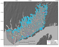
¹Data collected by National Oceanic and Atmospheric Administration.

²Data collected by U.S. Geological Survey

A seamless acoustic-backscatter image and digital elevation model (DEM) was also created. The backscatter mosaic GeoTIFF image for each source was resampled to 1 meter per pixel (to achieve a common resolution), and images were mosaicked together by using PCI Geomatica (version 10.1) (fig. 4).

Digital seismic-reflection data from surveys (fig. 5) completed between 2009 and 2011 (table 1) were loaded into a seismic interpretation software package, Landmark SeisWorks 2D (version R5000). The bulk of the data are chirp profiles from broadband frequencies of 4 to 24 kilohertz (kHz) and 0.5 to 12 kHz and a narrow-band 3.5-kHz system. A subbottom-profiling system with a boomer source and a multichannel (8 channels with a 3.125 m group interval) streamer was also used in selected locations. Legacy seismic-reflection data (Robb and Oldale, 1977; O’Hara and Oldale, 1980; McMullen and others, 2009) were used in the interpretation for a general confirmation and correlation of the seismic stratigraphy with previous studies. Seismic reflections (horizons) were identified and digitized in the time domain (two-way travel time), and seismic stratigraphic units were defined on the basis of their seismic facies.

High-density, seismic-reflection data did not extend beyond the USGS areas surveyed between 2009 and 2011 (table 1, fig. 5). As a result, surficial geology polygons derived from the seismic interpretations are not as extensive as the sea-floor sediment and physiographic zone polygons that incorporated the area of composite bathymetry (fig. 3). Therefore, one confidence level (high) was constant for the area of surficial geology and stratigraphic units mapped.

The thickness values of seismic units were calculated by subtracting the digitized sea-floor horizon from the subsea-floor horizons, exported difference in the time domain, and converted to thickness of the seismic-stratigraphic units in meters using a constant seismic velocity of 1,500 meters per second (m/s). The resulting thickness values were imported into ArcGIS (version 9.3.1) as point features (easting, northing, and thickness) and were gridded with 40-m cell sizes. Isopach grids were subtracted from the regional swath-bathymetry DEM (10-m cell size) to produce a DEM of the bounding unconformities (40-m cell sizes) relative to NAVD 88.

The digitized sea-floor outcrops for each seismic unit were imported into ArcGIS as point features (easting, northing, seismic unit) and used to guide manual digitizing of polygons representing discrete areas of seismic-unit outcrop. The resulting polygon dataset provides a seamless representation of surficial geology for the seismic-reflection survey area.

Surficial geologic maps derived from interpretation of the seismic profiles provided insight into the likely sediment texture at the sea floor on the basis of the glacial or postglacial (mostly marine) origin and depositional environment inferred from the seismic interpretation. This information was incorporated into the early stages of mapping the surficial sediment texture.

We used the Barnhardt and others (1998) sediment texture classification scheme (fig. 6). This scheme is effective for representing sea-floor texture of the New England inner-shelf environments where reworked glacial drift and rocky pavements are common. The Barnhardt and others (1998) classification defines surficial sediment types primarily on the basis of acoustic (side scan sonar) characteristics, which include reflectivity (backscatter), relief, and sea-floor features. The acoustic imagery shows lateral changes in the sea-floor character at small scales that would be largely undetected by grid-sampling methods. Barnhardt and others (1998) use geologic and geophysical data to correlate and support interpretation of the acoustically defined sea-floor units. Their classification scheme defines four basic, easily recognized sediment units: Rock (R), Gravel (G), Sand (S), and Mud (M). Because the sea floor is often a nonuniform mixture of these units, which are too small to define separately, the classification is further divided into twelve composite units, which are two-part combinations of the four basic units (fig. 6). The classification is defined such that the primary unit, representing more than 50 percent of an area's texture, is given an upper case letter, and the secondary texture, representing less than 50 percent of an area's texture, is given a lower case letter. If one of the basic sediment units represents more than 90 percent of the texture, only its upper case letter is used.

Using several data sources, including acoustic backscatter, bathymetry, seismic-reflection profile interpretations, bottom photographs, and sediment samples, we defined several regions of similar sediment texture on the Buzzards Bays sea floor. Polygons were digitized in Esri ArcMap to develop sea-floor texture maps by following methods similar to those used by Pendleton and others (2013). The sediment texture polygons were digitized at a scale between 1:5,000 and 1:20,000, depending on the resolution of the source data, but the recommended scale for application of these data is greater than 1:25,000. Supporting geologic information included sediment sample databases of Ford and Voss (2010) and McMullen and others (2011). These data included laboratory analysis of 325 samples with and the visual descriptions of 10,625 locations, some of which include NOAA chart sampling data (fig. 7; Massachusetts Office of Coastal Zone Management, unpub. data, 2012). In addition, we made observations from 1226 bottom photographs (fig. 7; Ackerman and others, 2014).

As was done in the mapping by Pendleton and others (2013), sediment texture polygons were assigned to one of four confidence levels (level one being highest) on the basis of the type and quality of data used to derive each polygon (table 2). The source data included swath, single-beam, and lead-line soundings; acoustic backscatter; seismic-reflection profiles; and either sediment samples with grain-size data from laboratory analysis or qualitative descriptions of sediment samples and bottom photographs. These confidence levels were attached as an attribute in the GIS for each sediment texture polygon (fig. 8). Confidence levels one and two were considered to have relatively high confidence. Level-one confidence areas contain the most varied and highest quality data (table 2). Level-two areas share the same levels of variety and quality but do not contain any sediment samples for which there is quantitative laboratory analysis. The absence of data with laboratory analysis was typical for areas that consist of gravel and gravelly sediment where no sediment sample was collected. Most bottom sampling methods are incapable of or inaccurate in sampling gravel and cobble. Level-three and -four areas have substantially lower confidence because the primary component of the Barnhardt and others (1998) classification, acoustic reflectivity, is lacking. Level-four-confidence areas only contain single-sounding bathymetry and have no supporting geologic information. Hereafter, confidence levels one and two are referred to as “high confidence”; levels three and four are referred to as “low confidence.”

Table 2. Confidence levels assigned to sediment texture polygons on the basis of the data used in the interpretation. The spatial distribution of polygons and associated confidence levels are shown in figure 8.

In high-confidence areas where we had acoustic backscatter (fig. 4), sediment texture polygons were digitized on the basis of backscatter intensity and patterns. Areas of high backscatter (strong acoustic reflectivity) suggest boulders, gravels, and generally coarse sea-floor sediments. Low-backscatter areas have weak acoustic reflectivity and are generally characterized by finer grained material such as muds and fine sands. Acoustic patterns seen in the imagery suggest common environments such as boulder fields, cobble pavements, sand sheets (with or without bedforms), and anthropogenic features.

The polygons interpreted from backscatter were then modified on the basis of sea-floor morphology from the bathymetry and bathymetrically derived data, which include slope, rugosity (small-scale changes in relief), and hillshaded relief maps. Areas of rough topography and high rugosity are associated with rocky areas, while smooth, low-relief regions tend to be blanketed by fine-grained sediment deposits. In low-confidence areas where backscatter data were not available, bathymetry and the bathymetric derivatives were used to create the initial polygons.

Sediment texture data and bottom photographs were used to verify and refine the classification of the sediment texture polygons. Samples with laboratory-analysis data rather than samples with qualitative descriptions were preferred for defining sediment texture throughout the study area. Bottom photographs were used to qualitatively define sediment texture, particularly in areas dominated by gravel- to boulder-size material. Many of the sediment type polygons do not contain sample information. For these polygons, sediment textures were extrapolated from proximal polygons that contained samples and had similar acoustic properties.

A stand-alone method was used to map bedrock outcrops from orthophotographs (Massachusetts Office of Geographic Information, 2001), and these mapped outcrops only represent those exposures visible at the sea surface.

Based on geologic maps produced for the western Gulf of Maine (Kelley and Belknap, 1991; Kelley and others, 1998; Barnhardt and others, 2006, 2009) and Massachusetts and Cape Cod Bay (Pendleton and others, 2013), the Buzzards Bay sea floor was divided into physiographic zones, which are delineated on the basis of sea-floor morphology and the dominant sediment texture. Physiographic mapping allows for efficient mapping of large areas in a readily useable format. The mapping physiographic zones does not require full data coverage and can be defined from a variety of data sources. These zones were defined qualitatively in ArcMap by using the same sources used to derive the sediment texture map. The polygons were assigned one of two levels of confidence, high or low, on the basis of the same criteria used in the sediment texture mapping (table 2).