 |
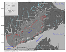
Figure 1. Location map of the Buzzards Bay study area, Massachusetts. Swath bathymetry, sonar backscatter, and chirp seismic-reflection data were collected in the area inside the red polygon. Dark gray is from a Massachusetts Office of Geographic Information (MassGIS) hillshade relief image of Massachusetts. Light blue lines show drainage modified from drainage of Massachusetts (MassGIS). Medium gray is the hillshade relief map modified from the composite bathymetry of Buzzards Bay (fig. 3). The light gray background indicates areas of ocean and coastal embayments where no hillshade relief image is shown. The Elizabeth Islands chain includes the islands labeled on the map: Nonamesset; Uncatena; Naushon; Pasque; Nashawena; Penikese; and Cuttyhunk. |
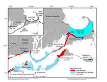 |
Figure 2. Map showing glacial moraines on land and submerged moraines (compiled from Stone and others, 2005; Boothroyd, 2008; Stone and DiGiacomo-Cohen, 2009; Stone and others, 2011) and ice-front locations (Ridge, 2004) for southern New England. Glacial Lake Cape Cod is shown with associated outlets (dark blue arrows), including the Monument River outlet (MRO) (modified from Larsen, 1982). Inset map shows locations of glacial lobes (modified from Oldale and Barlow, 1986). |
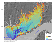 |
Figure 3. A digital elevation model (DEM) produced from swath interferometric, multibeam, and single-beam bathymetry at 10-meter horizontal resolution (table 1). Swath bathymetry data were collected in the area inside the red polygon. High rugosity and high relief are most often associated with rocky areas, whereas smooth, low-relief regions tend to be blanketed by fine-grained sediment deposits (fig. 17). The black rectangle indicates the location of figure 22. Depth is referenced to the North American Vertical Datum of 1988. |
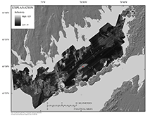 |
Figure 4. A composite backscatter image at 1-meter resolution was created from a series of published backscatter images (table 1). Areas of high backscatter (light gray tones) have strong acoustic reflections and suggest boulders, gravels, and generally coarse sea-floor sediments. Low-backscatter (dark gray to black tones) areas have weak acoustic reflections and generally indicate finer-grained material such as muds and fine sands. Red dot shows location of figure 20. |
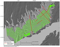 |
Figure 5. Map showing tracklines of chirp and boomer seismic-reflection profiles (table 1) used to interpret surficial geology and shallow stratigraphy. The bathymetry hillshade relief map is modified from the composite bathymetry of Buzzards Bay (fig. 3). |
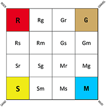 |
Figure 6. Barnhardt and others (1998) bottom-type classification based on four basic sediment units: Rock (R), Gravel (G), Sand (S), and Mud (M). Twelve additional two-part units represent combinations of the four basic units. In the two-part (composite) units, the primary texture (greater than 50 percent of the area) is given an upper case letter and the secondary texture (less than 50 percent of the area) is given a lower case letter. Figure is modified from Barnhardt and others (1998). |
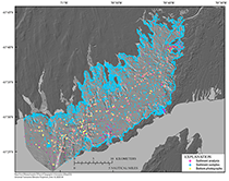 |
Figure 7. Map showing locations of bottom photographs and sediment samples collected within the study area to aid interpretations. Sediment samples analyzed in a laboratory are shown as magenta dots, whereas blue dots are locations of where samples have visual descriptions only (Ford and Voss, 2010; McMullen and others, 2011; Massachusetts CZM, unpub. data, 2012). Those processed in a laboratory to obtain grain-size statistics are preferred over those that were only described visually. Bottom photograph locations are generally associated with sites where samples were collected and grain-size statistics were processed. In rocky areas, visual descriptions were the only means to describe sea-floor sediments, as direct sampling was not possible given the large size of material on the seafloor. The bathymetry hillshade relief map is modified from the composite bathymetry of Buzzards Bay (fig. 3). |
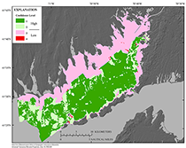 |
Figure 8. Map showing the distribution of confidence levels for sediment texture interpretation (table 2) within the Buzzards Bay study area. Confidence levels one and two (64 percent of total area) are significantly higher in confidence than confidence levels three and four. For that reason, this report describes areas in general terms of high confidence (levels 1 and 2) and low confidence (levels 3 and 4). |
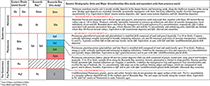 |
Figure 9. Seismic stratigraphic units and major unconformities interpreted within eastern Rhode Island Sound by O’Hara and Oldale (1980) and within Buzzards Bay by Robb and Oldale (1977) and by this study. |
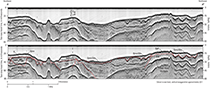 |
Figure 10. Chirp seismic-reflection profile A–A' with seismic stratigraphic interpretation. See figure 9 for descriptions of stratigraphic units and major unconformities. The red lines indicate reflections that bound seismic stratigraphic units (fig 9). See figures 16 and 18 for profile location. A constant sound velocity of 1,500 meters per second was used to convert two-way travel time to depth in meters. |
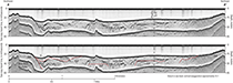 |
Figure 11. Chirp seismic-reflection profile B–B' with seismic stratigraphic interpretation. See figure 9 for descriptions of stratigraphic units and major unconformities. The red lines indicate reflections that bound seismic stratigraphic units (fig 9). See figures 16 and 18 for profile location. A constant sound velocity of 1,500 meters per second was used to convert two-way travel time to depth, in meters. |
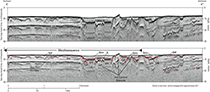 |
Figure 12. Chirp seismic-reflection profile C–C' with seismic stratigraphic and morphosequence interpretation (arrow pointing from ice-contact to ice-distal deposits). See figure 9 for descriptions of stratigraphic units and major unconformities. The red lines indicate reflections that bound seismic stratigraphic units (fig 9). See figure 16 for profile location. A constant sound velocity of 1,500 meters per second was used to convert two-way travel time to depth, in meters. |
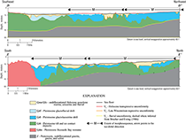 |
Figure 13. Geologic sections (D-D' and E-E') illustrating the general distributions and thicknesses of seismic stratigraphic units and major unconformities beneath Buzzards Bay. Geologic sections are interpreted from chirp and boomer seismic-reflection profiles. See figure 9 for descriptions of stratigraphic units and unconformities. Geologic section locations are identified on figure 16. |
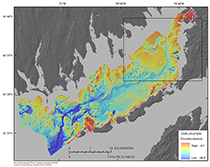 |
Figure 14. Map showing the elevation (referenced to the North American Vertical Datum of 1988) of the late Wisconsinan regressive unconformity Ur, which identifies the eroded surface of Pleistocene glacial drift beneath Buzzards Bay. Ur represents a composite unconformity where it locally merges with the Holocene transgressive unconformity (Ut) where wave-base erosion during the Holocene transgression truncated the lower unconformity, Ur. Black rectangle shows the location of figure 21. |
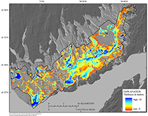 |
Figure 15. Map showing the thickness of postglacial fluvial and estuarine (Qfe) and nearshore marine (Qmn) sediments beneath Buzzards Bay. The black polygon depicts the boundary of the seismic-survey area. The bathymetry hillshade relief map is modified from the composite bathymetry of Buzzards Bay (fig. 3). |
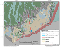 |
Figure 16. Map showing the surficial geology of Buzzards Bay with equivalent onshore glacial surficial geology (adapted from Stone and DiGiacomo-Cohen, 2009; Stone and others, 2011). The areal extents over which offshore subsurface geologic units crop out at the sea floor were interpreted from seismic-reflection data. See figure 9 for detailed descriptions of the offshore geologic units. Holocene sediment veneers too thin to be detected in the seismic-reflection data (less than approximately 0.5 m) might overlie outcrops of Pleistocene units locally. The bathymetry hillshade relief map is modified from the composite bathymetry of Buzzards Bay (fig. 3). Chirp profile locations are shown with black lines. Qmn/Qfe, undifferentiated Holocene nearshore marine and Holocene fluvial and estuarine; Qdt, undifferentiated Pleistocene glacial till and ice contact; Qdm, Pleistocene glacial moraine (Buzzards Bay moraine); Qdf, Pleistocene glaciofluvial (outwash and glaciodeltaic); Qdl, Pleistocene glaciolacustrine deposits (glaciodeltaic and lake floor). |
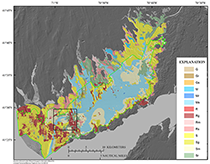 |
Figure 17. Map showing the distribution of sediment textures within the Buzzards Bay study area on the basis of the bottom-type classification from Barnhardt and others (1998) (fig. 6). The green polygon denotes higher confidence levels (fig. 8; table 2) inside the green line and lower confidence levels outside the green line. The black rectangle indicates the location of figure 18. The bathymetry hillshade relief map underlying the sediment texture layer is modified from the composite bathymetry of Buzzards Bay (fig. 3). |
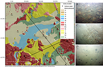 |
Figure 18. A, Sediment textures within an approximately 6.5- by 6-kilometer area in western Buzzards Bay (see fig. 17 for location). The bathymetry hillshade relief map underlying the sediment texture layer is modified from the composite bathymetry of Buzzards Bay (fig. 3). The pink polygons separate areas of high confidence level (larger area) from low confidence level (smaller areas). The location of seismic profiles A–A' and B–B' from figures 10 and 11 is shown here. B, A photograph of the sea floor showing a gravel-cobble pavement within an area classified as rock with gravel (Rg), which corresponds with areas of high rugosity. C, A photograph of a section of sea floor classified as primarily rock with sand (Rs). D, A photograph from a section of sea floor classified as primarily sand with some mud (Sm). The viewing frame for photographs B–D is approximately 50 centimeters, and the locations of the photograph transects are shown as red dots in map A. |
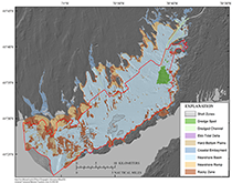 |
Figure 19. Map showing the distribution of physiographic zones within the Buzzards Bay study area. The physiographic zone classification is adapted from Kelley and others (1998), and the zones are delineated on the basis of sea-floor morphology and the dominant texture of surficial material. The red polygon denotes higher confidence levels (fig. 8; table 2) inside the line and lower confidence levels outside the line. The bathymetry hillshade relief map underlying the physiographic zone layer is modified from the composite bathymetry of Buzzards Bay (fig. 3). |
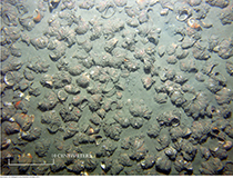 |
Figure 20. Bottom photograph showing mud with sand sediment texture and high concentrations of Crepidula fornicata. The photograph was taken in an area of high acoustic backscatter. See figure 4 for photograph location. |
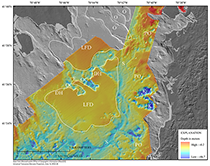 |
Figure 21. Map showing detailed area of depth to the top of glacial deposits (fig. 14). The gray bathymetry hillshade relief is modified from the composite bathymetry of Buzzards Bay (fig. 3). These surfaces show the morphology of glacial outwash and associated features. Lacustrine fan deltas (LFD) and coalescing outwash lobes (O) are outlined in white. Outwash channels (OC) and the delta head (DH) are labeled on the well-preserved LFD in the center of the basin. This feature is considered to be a single ice-contact lacustrine delta morphosequence on the basis of the interpretation of the chirp profiles (fig. 12). An esker (E) separates the outwash channels. Spillways (S) indicate where proglacial lakes drained. Pitted outwash (PO) and large kettles (K) are along the eastern shore. See figure 14 for map location. |
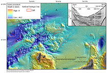 |
Figure 22. Map showing bathymetry and areas of erosion. The hillshade relief map underlying the bathymetry layer is modified from the composite bathymetry of Buzzards Bay (fig. 3). A, striations on the sea floor are truncated estuarine and marine sediment. B, scour depressions where glaciolacustrine deposits (Qdl) are exposed at the sea floor. See figure 3 for location of this map. Inset is a chirp seismic-reflection profile that shows truncation and exposure of glaciolacustrine (Qdl) deposits in a scour depression north of Quicks Hole (green line). |

