Figure 4. Maps showing A, acoustic backscatter data collected using the multibeam echosounder in 2014 (Denny and others, 2015) and B, transitions and distances between areas of high- and low-backscatter margins of common sea-floor features digitized from 2011 (Schwab, Denny, and Baldwin, 2014) and 2014 backscatter data. C, Graph illustrating the mean movement (in meters) of backscatter transitions within four depth intervals between 2011 and 2014. Vertical bars indicate one standard deviation of mean value.

Figure 5. Maps showing A, backscatter and B, bathymetry collected in 2011 (Schwab, Denny, and Baldwin, 2014) and 2014 (Denny and others, 2015) in the vicinity of a borrow pit offshore of western Fire Island, New York. Location of maps shown on figure 4B. A, Sharp transitions between areas of high and low backscatter identified along the margins of discrete sediment distribution patterns, bedforms, and sedimentary structures from the 2011 and 2014 surveys are overlain on the backscatter data from the 2014 survey. B, Bathymetric data from each survey also illustrates significant change around the borrow pit area.

Figure 6. Maps showing A, backscatter and B, bathymetry collected in 2011 (Schwab, Denny, and Baldwin, 2014) and 2014 (Denny and others, 2015) in an area of sorted bedforms offshore of eastern Fire Island, New York. Location of maps shown on figure 4B. A, Sharp transitions between high and low backscatter identified along the margins of discrete sediment distribution patterns and sedimentary structures from the 2011 and 2014 surveys are overlain on the backscatter data from the 2014 survey and aid in detecting change. B, Coincident bathymetry illustrates that change detection is prohibitive largely because of the subtlety of changes in this area. Change detection is further complicated because of artifacts in the data from the 2011 survey as described in the “Methods” section of this report.

Figure 7. Map showing change in modern sediment thickness in meters between the 2011 (Schwab, Baldwin, and Denny, 2014) and 2014 surveys. A vertical resolution of 20 centimeters (cm) is assumed for the sediment volume calculation because of the resolution limits of the seismic system used. However, the change in sediment thickness is displayed with a less conservative estimate of 10 cm to better illustrate the sediment flux patterns. It is assumed that the majority of this change was a result of Hurricane Sandy.

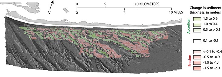
Methods

Data Acquisition and Processing

The study area (fig. 1) was surveyed in May 2011 aboard the motor vessel Scarlett Isabella using an interferometric sonar to acquire bathymetric and acoustic backscatter data and a chirp seismic-reflection profiler to define the subsurface stratigraphy and structure. The survey area extends about 50 kilometers (km) alongshore and about 8 km offshore in water depths ranging from approximately 8 to 32 meters (m), covering approximately 336 square kilometers (km²). A full description of the acquisition and processing of these data is provided in Schwab, Denny, and Baldwin (2014).

The study area offshore of Fire Island was resurveyed in January to February 2014 (fig. 1) aboard the research vessel Shearwater using a multibeam echosounder to acquire bathymetric (fig. 2A) and backscatter data (fig. 4). Details of the acquisition and processing of these data are described in (Denny and others, 2015).

An area about 86 km² of prominent shoreface-attached sand ridges offshore of western Fire Island was resurveyed in October 2014 (fig. 1) using the same high-resolution seismic-reflection system used in 2011 to reassess subsurface stratigraphy and structure. The methodology used for data collection, navigation, and processing of seismic-reflection data was identical to that used in the 2011 survey (Schwab, Denny, and Baldwin, 2014). Survey line spacing varied from approximately 75 to 300 m.

Change Analysis

The acoustic backscatter data from the 2011 (Schwab, Baldwin, and Denny, 2014) and 2014 surveys (Denny and others, 2015) were compared to assess morphologic changes before and after major storms on the inner continental shelf. This analysis involved identifying discrete sea-floor features common to both datasets, but perhaps in different locations, by manually digitizing within a geographic information system (GIS) sharp transitions between high and low backscatter along their margins, indicating variation in sediment texture and (or) structure (fig. 4). The digitized transitions for each survey period were stored in a GIS feature class. Additional lines were then digitized between common feature boundaries at roughly perpendicular angles and equal intervals along the lengths of the lines to evaluate lateral offset distances between the locations before and after these major storms (figs. 5 and 6). Basic spatial and statistical analyses were used to assess variability in the magnitude of boundary movements with respect to water depth. Depth contours produced from the bathymetric data from the 2014 survey (fig. 2B) were used to spatially query the lateral offset distance lines contained within the areal bounds for four 5-m depth intervals (10 to 14.9 m, 15 to 19.9 m, 20 to 24.9 m, and 25 to 29.9 m). Minimum, maximum, mean, and standard deviation statistics were produced for the lateral offset distance line subsets from each depth interval (fig. 4C).

Changes in modern sediment thickness on the inner continental shelf before and after major storms were evaluated by comparing isopachs produced from interpretations of the seismic-reflection data from the 2011 (Schwab, Baldwin, and Denny, 2014) and 2014 surveys (fig. 2). Sediment thicknesses were mapped following the methods described by Schwab, Denny, and Baldwin (2014), in which along-track two-way travel times between the sea floor and the Holocene transgressive unconformity horizon were converted to thicknesses, assuming an internal seismic velocity of 1,500 m/s. The computed along-track sediment thickness values were then interpolated using the natural neighbors algorithm of ArcGIS Spatial Analyst to create 50-meter-per-pixel-gridded isopachs for each survey. The isopach from the 2011 survey (Schwab, Baldwin, and Denny, 2014) was then subtracted from the isopach from the 2014 survey using the raster calculator of ArcGIS Spatial Analyst, yielding a 50-meter-per-pixel-difference grid to illustrate areal patterns of accretion and erosion during the 3-year period within the area common to the two surveys (fig. 7). A vertical resolution of 20 centimeters (cm) is assumed for the sediment volume calculations because of a conservative estimate of the vertical resolution limits of the subbottom profiling system used. However, the change in sediment thickness shown in figure 7 was created using a less conservative vertical resolution of 10 cm to better illustrate net sediment flux.

A comparison of the swath bathymetric surfaces from the 2011 (Schwab, Denny, and Baldwin, 2014) and 2014 (Denny and others, 2015) surveys also clearly identifies geomorphic changes in places (fig. 5B), but quantifying that change at the regional scale is not possible because of the vertical resolution limitations of the swath bathymetric systems used. Although the interferometric sonar data from the 2011 survey and the multibeam echosounder data from the 2014 survey show decreased signal-to-noise ratio in the far range, the interferometric sonar data from the 2011 survey show additional data loss in the far range because of interference from the ship’s hull and errors introduced because of a lack of sound velocity profiles needed to accurately correct refraction artifacts present in the data (Schwab, Denny, and Baldwin, 2014).