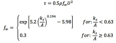
Data Processing

Water Velocity and Calculated Shear Stress from Acoustic Profiler

            The Vectrino acoustic velocity profiler measured 3D water velocity of a 4-cm profile below the instrument with 1-mm-spaced bins and the distance from the instrument to the sand bed using coherent Doppler processing at a frequency of 100 Hertz. Initially, profiler log data were extracted with MathWorks Matlab (MathWorks, Inc., ver. 2015b, 2015). Raw velocities were then passed through a modified PST (phase-space thresholding) spike removal filter. The mean square and root mean square of both raw and filtered velocities were calculated and initially saved in Matlab data files, which were later converted to text files of velocity time series as presented in the Data Catalog section of this report. Time series of flow-velocity profiles were returned at a sampling rate of 100 Hz.

Velocities were passed through a Matlab built-in one-dimensional digital smoothing filter (filter.m) with a window size of 10. For incipient motion experiments, instantaneous shear stress (τ) was calculated using equation 1 (Soulsby, 1997), along with high-, medium-, and low-critical stresses, as calculated in Plant and others (2013). The roughness used in calculated exerted stress is taken as 2.5 times the diameter of the aSOA in order to approximate the skin friction force acting on the aSOA to drive incipient motion. Velocities used were taken from the fifth bin below the instrument:

where τ is shear stress, ρ is density of water, f_w is the wave friction factor, U is water velocity, k_s is 2.5 times the diameter of the aSOA, and A is the orbital excursion amplitude, which was set equal to the flywheel stroke length based on the assumption that the flow velocities generated in the tunnel are equivalent to those generated by a monochromatic wave. This assumption was verified by performing spectral analysis on the measured velocities to calculate the orbital excursion amplitude in the tunnel. The measured excursion was approximately equal to the stroke length within estimated error.

Image Processing and Movie Creation: False Floor Experiment

Image processing was handled using Mathworks Matlab with the Image Processing toolbox and the California Institute of Technologies Camera Calibration Toolbox (MathWorks, Inc., ver. 2015b, 2015). A single extracted frame from video footage of a 2-cm-spaced black-and-white checkerboard placed in the S-OFT was used as a calibration image to assign real-world (x-z) coordinates (mm) to each pixel in the raw video data (fig. 7). The corners of the checkerboard squares were automatically extracted, creating a grid relative to the laser-line position points. Individual still-frame images were extracted from the raw video footage for each experiment at the native frame rate (30 fps) with no averaging or frame loss. Matlab algorithms then extracted the location of the laser line from each image based on the local maxima in image color contrast, which produced a time series of the laser-line position in pixel coordinates. Outliers caused by dust particles and stray bubbles were removed. Finally, the laser pixel coordinates were transformed to the real-world (x-z) coordinates (mm) of the laser-line position and were interpolated from the calibration grid. Additional options were available in the software for removing the image distortion caused by short (<20 mm) focal lengths, but were deemed unnecessary for incipient motion, as only change detection, not actual position, is needed for the calculations. The noise in the laser data was too high, particularly for smaller size aSOAs, for automated incipient motion detection. Therefore, laser-line position data were used to manually select the instantaneous aSOA incipient motion from video data. Incipient motion times were selected based on careful visual inspection of each experimental video, including experiments where laser data were not available.

Movies of aSOA incipient motion video paired with a plotted time series of calculated stresses were created using Mathworks Matlab (MathWorks, Inc., ver. 2015b, 2015).  Velocity and video data were time matched and time periods around the instantaneous time of incipient motion for single aSOA objects were isolated. The time window around the instant of incipient motion was limited by Matlab software to 42 seconds, with 30 seconds prior to and 12 seconds following incipient motion, except when motion occurred near the beginning or end of an experiment run. The videos were time synced to the Vectrino time during the experiment. During the experiment, a red LED light was place on the tank and flashed only once at the instant the Vectrino began recording data. The corresponding frame was identified from the video stills for each experiment, which allowed the velocity and video data to be synchronized. Paired motion and stress movies were then compressed using free compression software, Avidemux, and are provided in the Data Catolog section of this report.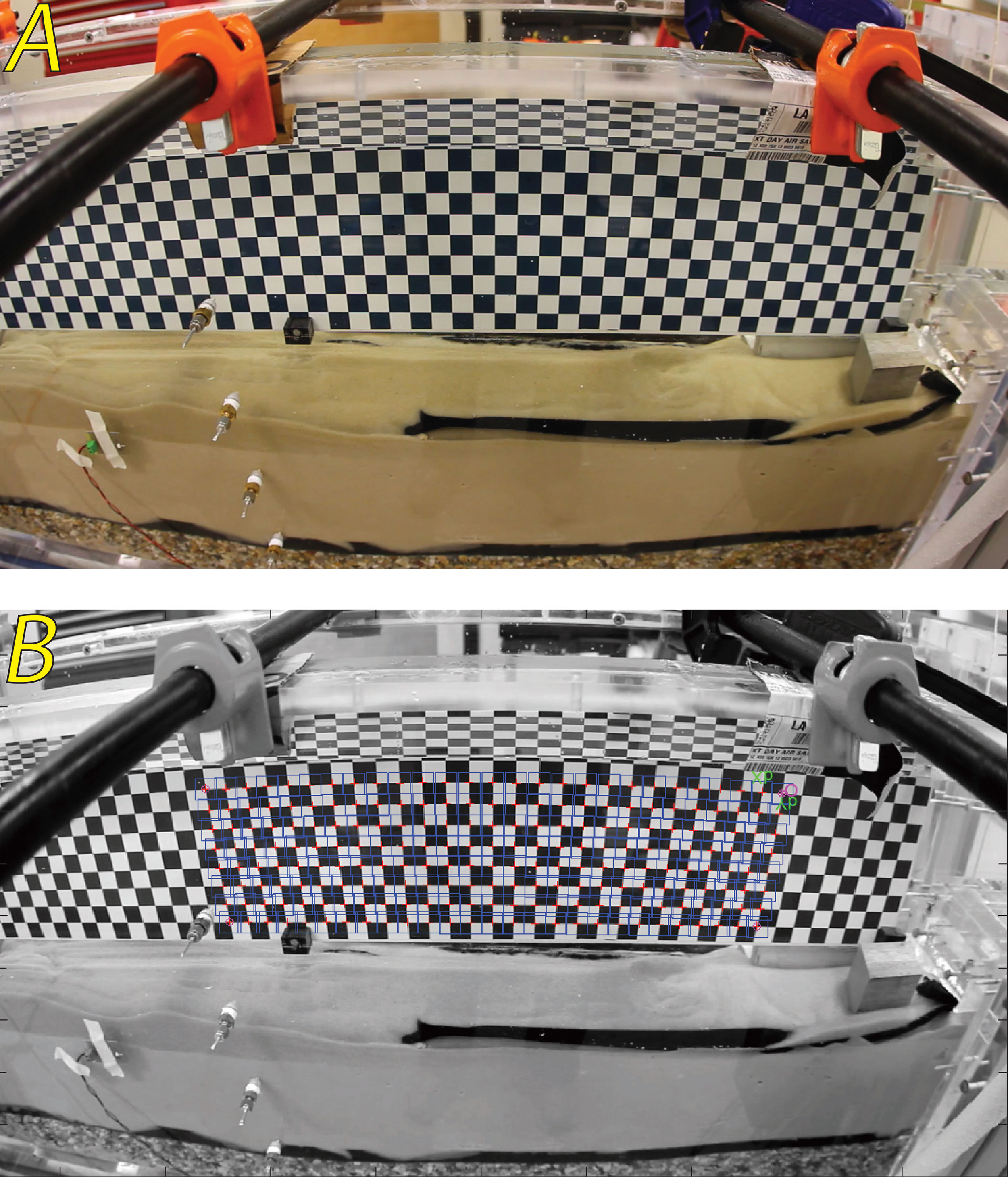

Figure 7. Photographs of reference checkerboard placed in the tank after the experiments (A) and the automatically extracted grid corners found during image processing (B). The checkerboard serves as a calibration to give x-z, real-world reference points to each image pixel for laser-line position measurements. [Click figure to enlarge]

Image Processing and Movie Creation: Moving Bed Experiment

Frames were extracted from the HD video data for this set of experiments, and movies of the results were created using the Matlab Image Processing Toolbox, showing aSOA motion along with time-synced velocity. Because critical stress and shear stress exerted on the aSOAs depends on their size, and multiple sizes were included in these experiments, a time series of stress is not included in the videos. Videos for each experiment were then compressed using Avidemux software to minimize storage-space requirements. Qualitative descriptions of this video data are available in the Results section of this report. Descriptions of each experiment, along with links to the videos, are presented in the Data Catalog.