The following figures are in PDF format. Figure 4A Figure 4B Figure 16A Figure 16B Figure 17 Figure 18 Figure 19 Figure 20 Figure 21 Figure 22 Figure 23 Figure 24

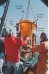
A variety of sensors were used to measure current, temperature, conductivity, light transmission, oxygen, and pressure; these sensors were deployed on a variety of platforms (table 3 and descriptions below).  The data from these sensors were sampled and recorded by various data logging systems (table 4).

Most of the current and pressure measurements were obtained using a burst sampling scheme to average out, or in some cases to measure, high-frequency fluctuations, caused primarily by surface waves. In a burst scheme, samples are obtained at a fast rate (typically 0.5-2 Hz for the data in this report) over a time interval (typically a few minutes); the burst is repeated at a second interval (typically 1 to 10 minutes for the data here). Averaging the data from the burst samples provides a measure of the mean value of the variable over the burst duration, and statistics from the burst samples can provide a measure of the high-frequency fluctuations. Burst sampling schemes are used to conserve power and data storage in instruments but, as instrument capabilities have increased, the duration of the burst has increased in length. Internal processing capabilities in some instruments enable them sample nearly continuously and average the data in the field. Increased data storage capacity has also made it possible for instruments to save high-frequency measurements.

Sea-floor Tripod Systems (fig. 4A, 4B, 16A, 16B, 17)

USGS tripod systems provide a platform for long-term deployment of instruments to measure currents and water properties near the sea floor. These observations are of particular interest in studies of sediment resuspension and transport. At LT-A, instruments deployed on a large tripod frame (fig. 4A) measured currents about 1 m above bottom; temperature, pressure, light transmission, and conductivity about 2 m above bottom; sediment-collection rate at 1 and 2 m above bottom; and current throughout the water column, and photographed the sea floor. At LT-B, instruments deployed on a smaller frame (fig. 4B), which measured currents throughout the water column, and temperature, salinity, and sediment-collection rate about 1 m above bottom. For the Massachusetts Bay long-term observations, the tripod systems were deployed for about 4 months and data were recorded internally.

During 1989-2006, three data-logging systems were used to obtain the near-bottom observations at LT-A. From 1989 to 1991, a Data Logging Current Meter (DLCM) system was used that measured current with two Savonius rotors and a vane. The DLCM recorded data on a pair of Sea Data tape cassettes or to a hard disk using an Onset Computer Tattletale computer (Butman and Folger, 1979). The DLCM tripod system recorded averages of rotor speed and pressure every 7.5 minutes. Measurements of temperature and conductivity were made at the midpoint of the averaging interval. The instrument also burst-sampled current speed, current direction, and pressure every 2 seconds for 72 seconds (180 seconds if recording on a Tattletale) at the midpoint of each 7.5-minute interval. When the DLCM data were processed, the burst current measurements were vector-averaged to obtain current speed and direction, and the standard deviation of the high-frequency pressure measurements, called PSDEV, was computed as a measure of the bottom-pressure fluctuations caused by surface waves.

From 1991 to 2003, near-bottom observations at LT-A were made with a MIDAS system that measures current with two BASS (Benthic Acoustic Stress Sensor) four-axis acoustic current sensors (fig. 16A, 16B) mounted nominally at 1.0 and 0.45 m above bottom. Data were recorded using a Tattletale computer (Martini and Strahle, 1992). The MIDAS system recorded pressure and four velocity components from each BASS current sensor (Williams, 1985) at 1 hz. Every 3.75 minutes, MIDAS computed cumulative sums of pressure and current and recorded them, along with values of temperature, conductivity, and light transmission measured at the midpoint of the 3.75-minute averaging interval. Average pressure and current were calculated during data processing.

BASS current meters can resolve 0.0003-m/s currents; however, this resolution requires a field determination of the zero. Accuracy is affected by the capacitance of the cables that connect the data logger to the sensors which change with each deployment; therefore a new calibration must be obtained each time the data logger and sensor wiring are attached to a tripod frame. An accuracy of 0.003 m/s can be achieved when the offsets generated by these capacitance changes are measured and removed from the data. The BASS current-meter voltages were measured when there was no current through the measurement volume, and this 'zero' offset was subtracted from measurements made during the deployment. A set of experiments was performed to determine the most efficient method of calibrating the BASS to 0.003 m/s accuracy (Morrison and others, 1993). A zero calibration for the BASS current sensors was obtained with the sensors mounted on the tripod system and connected to the MIDAS data logger prior to deployment and after recovery. A water-tight jacket was fitted around the two BASS sensors and filled with water, and data were recorded for at least 12 hours to determine an offset under no-flow conditions.

The MIDAS system measures conductivity using a Sea-Bird SBE-4 conductivity cell (fig. 17), the same sensors used by Sea-Bird's SEACAT and MicroCAT data loggers described below. On stationary near-bottom platforms such as the tripod, sediment can collect in the conductivity cell and bias the measurement. In the middle 1990's, this sediment accumulation was suspected to be the cause of a consistent freshening trend over the course of a deployment observed in the conductivity data collected from instruments mounted on the tripods. Sea-Bird pumps were added to the MIDAS to flush the conductivity cell prior to making a measurement.

In 2003, the MIDAS loggers and BASS current sensors were retired, and near-bottom velocity measurements were made with a Sontek Acoustic Doppler Velocimeter (ADV)

Camera (fig. 18)

A 35-mm Benthos camera system was mounted on the tripod frame approximately 2 m above the bottom (fig. 18) and programmed to take a single photograph of the sea floor every 4 hours. The field of view of the downward-looking camera was approximately 1 m by 1.5 m. The photographs are published in separate data reports (Butman and others 2008a, 2008b).

Acoustic Doppler Current Profiler (ADCP) (fig. 19)

ADCPs made by RD Instruments (a 300-kHz Workhorse) were deployed at LT-A beginning in 1994, and at LT-B beginning in 1997 to obtain profiles of currents throughout the water column. The instruments measure currents from the Doppler shift of sound reflected from the water column from two pairs of orthogonal acoustic beams (fig. 19). The instruments recorded 5-minute averages of current every 15 minutes. To obtain an accuracy of at least 0.004 m/s for each 5-minute measurement, 300 pings emitted at a rate of 1 ping per second were averaged together. At LT-A, the ADCP was deployed on a small tripod frame (fig. 4B) from 1994 to 1996 and on the large frame beginning in 1996 (fig. 4A). At LT-B, the ADCP was deployed on several versions of a small tripod frame (fig. 4B, fig. 19).

Vector-Measuring Current Meter (VMCM) (fig. 20)

Vector-measuring current meters (Weller and Davis, 1980) were used to measure temperature and velocity at a sampling interval of 3.75 minutes (fig. 20). At LT-A, VMCM's were maintained on subsurface moorings at a depth of about 22 m (10 m above bottom). VMCMs were also suspended from the 40-ft discus buoy, at a depth of 5 m below the surface, from December 1989 until February 1994 when the buoy was discontinued. VMCMs use orthogonal bidirectional propellers and were configured to sample the currents every 0.25 seconds and vector-average internally to calculate averages at the sampling interval of 3.75 minutes. Beginning in 2002 (mooring 696), new versions of the VMCM electronics measured current and temperature every 60 s.

SEACAT (fig. 21)

SEACAT 16 instruments (http://www.seabird.com/) measure conductivity and temperature, and record the voltage signals produced by a transmissometer. SEACAT's were operated with a sampling interval of 3.75 minutes. SEACATs were attached to the VMCMs that were maintained on subsurface moorings at a depth of 22 m (10 m above bottom), as well as to the VMCMs that were suspended below from the 40-ft USCG discus buoy, at a depth of 5 m, from December 1989 until February 1996. Concern that the SEACAT batteries might be disturbing the VMCM compasses led to a change in mooring design in February 1998, after which the SEACATs were attached to the moorings immediately above the VMCM at a depth of 21 m (11 m above bottom).

MicroCAT (fig. 22)

The MicroCAT is a simple version of the SEACAT 16. The MicroCAT uses the same sensor technology as the SEACAT to collect salinity and temperature data but cannot record data from additional external sensors such as transmissometers. MicroCATs were attached to the top floats of the subsurface moorings at LT-A and LT-B. The recording interval was matched to the other instrumentation, typically every 3.75 minutes.

Transmissometer (fig. 23)

Sea Tech transmissometers measure the transmission of red light (wavelength 650 nm) from a Light Emitting Diode (LED) along a 25-cm water path. The voltage output by a photovoltaic detector was recorded by a SEACAT or by a logging system on a tripod. Biological fouling of the transmissometer windows often limited the usefulness of the observations. From October 1992 to October 1994, tests of anti-fouling rings fitted around transmissometer windows showed some reduction in biological fouling (Strahle and others, 1994). Anti-fouling rings were used on all transmissometers beginning in 1994. Because of changing particle characteristics and fouling of the optical windows, the light transmission observations provide only a qualitative indication of suspended-sediment concentration.

Acoustic Doppler Velocimeter (fig. 4A)

An ADV measures current speed and direction at a single point in a sampling volume of approximately 2 cm³ using the Doppler principle and the difference between signal returns at the three receivers. The instrument can measure currents and pressure at high frequencies in multiple sampling schemes and rates, and store the complete raw data set. The ADVs are typically mounted on tripods facing downward. They are unique in their ability to measure three components of flow with accuracies of less than 0.003 m/s at rates of up to 25 Hz. At LT-A, the ADVs were typically set to measure for 3 minutes at 2 Hz every 5 minutes.

Sediment Traps

Time-series sediment traps (fig. 3, 24)

A time-series sediment trap (model MK 78HW-13) is manufactured by Mclane Research Laboratories, Inc., East Falmouth, Mass. The function and design of the instrument are described by Honjo and Doherty (1988). It consists of a polyethylene funnel 106 cm long with an 80-cm-diameter mouth. The open end of the funnel is fitted with a honeycomb-shaped baffle made of polycarbonate hexagonal cells 3.2 cm in diameter and 7.5 cm long. Covering the baffle is a polyethylene screen (1-cm mesh). The purpose of the baffle and mesh is to reduce turbulence and resuspension in the funnel and to keep out fish and other organisms that are known to take up residence in open traps. Excluding macrofauna from the trap minimizes their direct contribution of excretion products to the sample.

The funnel directs particulate matter into one of thirteen 500-mL plastic bottles, which are threaded into a rotating plate under the funnel. Each bottle is advanced to the sampling position under the funnel on a selectable schedule assigned using an internal Tattletale 8 computer. The sampling interval for each bottle is typically about 10 days for a 4-month deployment. Samples are sealed except for the period during which they are under the funnel. To reduce the decomposition of organic matter in the period between collection and analysis, each bottle is filled with a solution of 5-percent sodium azide (NaN₃) in filtered seawater before deployment. The higher salinity (and density) of the azide solution compared to ambient seawater significantly reduces its diffusion out of the trap during the 4-month collection period.

Although this trap was originally designed for long deployments in the open ocean, the size of the funnel mouth and the bottle volume are appropriate for 4-month deployments at 4.5 m above bottom in this coastal setting (water depth 30 m). Typically, there was a measurable amount of sediment (more than 0.1 g) in each bottle, even during quiet periods in summer when resuspension events are infrequent. Occasionally, during an unusually strong storm, the magnitude of sediment resuspension was so great that a sampling bottle overfilled and sediments accumulated in and plugged the throat of the funnel. Under these conditions the remaining bottles were empty when the trap was recovered. The bottles from each deployment were photographed to show visually the changes in collection rate during the deployment period.

Tube sediment traps (fig. 3, 24)

Traps made from standard core tubing were also used on the USGS moorings in order to obtain samples at multiple levels in the water column. These traps consist of a 60-cm-long polybutyrate tube with a 6.6-cm internal diameter and a wall thickness of 3.2 mm. The bottom of the tube was sealed with a securely taped plastic cap. Baffles consisted of an aramid fiber phenolic resin honeycomb (trade name Hexcell) with a cell diameter of 1 cm and a length of 7.5 cm. The material showed no apparent deterioration during exposure to seawater, although it is subject to bio-fouling. The tube traps are inexpensive to construct and are easily attached to other instruments or to the mooring wire with black electrical tape.

To accommodate different chemical analyses of the sediment samples, different preservative solutions were used with little effect on the collection rate. Most traps were filled to within 7.5 cm of the top with a filtered solution of 5-percent sodium azide in seawater. Some traps at the same location and depth had no preservative, and others were filled with a filtered solution of seawater containing 2-percent formaldehyde, 0.1-percent sodium borate and an additional 35 g/kg NaCl. The average standard deviation of the trapping rate for the three conditions (azide, formalin, and no poison) was 5 percent of the mean value. This result indicates that the density gradients in the traps below the Hexcell baffle had little effect on the trapping dynamics of the tube traps.

Trapping efficiency is a factor that must be considered if the results from the tube traps and the time-series traps are compared. A number of studies have discussed the dependence of aspect ratio (height/width), shape, tilt, Reynolds number (UD/k, where U = horizontal fluid velocity, D = trap diameter, and k = kinematic fluid viscosity) and other factors (Butman, 1986; Gardner, 1980, 1986). In this study, relative trap efficiency was compared during a number of field experiments by simply comparing the collection rates in the time-series traps with those in tube traps fixed at the same location and depth. A summary of the data since 1989 indicates that time-series traps collect at a lower rate than tube traps by a factor of 0.28 +/-0.11. This difference is consistent with a comparison of efficiency between tube traps and funnels up to 50 cm in diameter conducted on the edge of the continental shelf (Bothner and others, 1988).

Oxygen Sensors

Endeco Type 1184

The Endeco 1184 dissolved oxygen and temperature recorder was a microprocessor controlled, pulsed polargraphic oxygen sensor (Clark Cell) filled with electrolyte and covered with a one-mil thick teflon membrane (Endeco, 1988). It was designed for stable, long term measurements of dissolved oxygen in marine environments. The accompanying thermistor installed adjacent to the oxygen sensor was a single bead thermistor sheathed in a stainless steel tube.

Aanderaa optode

The Aanderaa optode (model 3830) is an optical sensor. It uses a micro-optode that measures fluorescence lifetime quenching using a sensing foil developed by Precision Sensing GmbH. Chemicals in the foil are excited by light of a certain wavelength, and the duration of the emissions is a measure of the oxygen content in the water. The accuracy of the Aanderaa optode is specified as 0.18 mL/L, with a resolution of 0.02 mL/L and an equilibration time of less than 25 s. The Aanderaa optode is intended to remain stable and accurate for a period of one year before a new two-point calibration and replacement of the foil are required. The foil is held in place by a window-frame surround. Fouling may be inhibited by the installation of a copper surround instead of the standard plastic material. Martini and others (2007) compare the performance of the Aanderaa Optode and Sea-Bird SBE43 sensors.

The Sea-Bird SBE43

The Sea-Bird SBE43 oxygen sensor uses a membrane polarographic oxygen detector, an upgraded Clark cell, redesigned and optimized to reduce drift and hysteresis effects (Carlson 2002; Sea-Bird Electronics, Inc., 2002a). The accuracy of the Sea-Bird SBE43 is 2 percent of saturation (Sea-Bird Electronics, Inc., 2005), and the measurements are stable to within 2 percent of calibration per 1000 hours if the membrane is kept clean and moist. The sensor requires 30–36 s to equilibrate (Sea-Bird Electronics, Inc., 2002b). Flushing of the sensor is required to achieve the specified accuracy and measurement stability; otherwise, the oxygen in the measurement volume would be depleted. Sea-Bird recommends that the SBE43 be recalibrated after every long-term in-situ deployment. Fouling may be inhibited by application of tributyl-tin leaching tips on the intake and discharge of the sensor. Martini and others (2007) compare the performance of the Aanderaa Optode and Sea-Bird SBE43 sensors.

Back to top of page

To view files in PDF format, download free copy of Adobe Reader.