By Scott T. Prinos

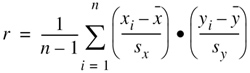
CORRELATION ANALYSIS OF A GROUND-WATER LEVEL MONITORING NETWORK

Analysis Methodology

The data from the continuous ground-water level monitoring network consist of daily maximum water levels. The water-level data were subdivided into wet season (June to October) and dry season (November to May) by water year. For the purposes of this report, the period November 1 to October 31 constitutes a water year. This is slightly different than the water year defined for other USGS reports (October 1 to September 30), and it is based on the consideration that about 70 percent of the annual rainfall in Miami-Dade County occurs during the wet season from June to October. The correlation analysis was performed for the period November 1, 1973, to October 31, 2000 (water years 1974-2000).

For the monitoring wells examined, the amount of data available for the period analyzed ranged from about 2 to 27 years and averaged about 17 years. Completeness of water-level data ranged from 38 to 100 percent and averaged 96 percent (table 2). Some stations were missing large percentages of water-level data because they had been discontinued for a number of years and then reactivated. Many of the wells in the vicinity of the West Well Field (figs. 1 and 2) were installed in 1994 and have only about 7 years of available data because they were installed in 1994.

The correlation analysis was performed using S-PLUS 2000 statistical software. The S-PLUS statistical function "Cor" was used to provide correlation matrices. When the data evaluated are not trimmed, this function yields the standard Pearson sample correlation coefficient (MathSoft Inc., 1999). The Pearson test yields the test result r, which is defined as:

,

where xi and yi represent corresponding values from the data sets being compared, and represent the means of each data set, and s_x and s_y are the sample standard deviations of each data set (Helsel and Hirsch, 1992). As previously discussed, the Pearson test assesses linear correlation.

A series of scripts were written to determine the extent of correlation between the water-level data of each network well and that of all other network wells for equivalent periods of record. For each network well, the correlation coefficient for the comparison of its own water-level data and that of all other network wells was determined for each season and year. The resulting correlation values were averaged to provide matrices for all of the wells examined for the wet and dry seasons for the period analyzed (app. I and II, respectively). The number of seasons used to determine each average correlation coefficient and standard deviation of the correlation coefficients for the period compared also were determined and included in the matrices.

The issue of missing water-level data in the correlation analyses can be addressed in one of two ways: (1) the correlation coefficient can be considered invalid if any amount of water-level data is missing, or (2) the coefficient can be determined using all available data. Because short periods of missing water-level data are common in ground-water wells, it is impractical to require a complete data set. Therefore, this analysis used a mathematical process for which all of the water-level observations available from the wells were compared. This is a more complex calculation than the standard Pearson analysis. When this option for handling missing observations is implemented using S-PLUS 2000 analytical software for a data matrix x with columns i and j, the means and the variances are computed for each variable using all available observations. The covariance for each pair of variables was then computed using the available observations for that pair. The divisor for the covariance of x[,i] and x[,j] was:

N[i,j]-1+(1-N[i,j]/N[i])(1-N[i,j]/N[j]),

Using this mathematical process, correlation coefficients outside the range -1 to 1 can be determined. To determine reasonable correlation coefficients, while at the same time allowing for some missing water-level observations, seasons were not considered for which one of the wells being compared was missing more than 5 percent of the data.

Irregularities in the data could be partly addressed by computing a trimmed correlation coefficient. This method of analysis can automatically censor a specified fraction of the highest and lowest data points. Trimmed correlation coefficients were not computed because data used for this analysis had already been reviewed and edited manually.

The amount of data available for the period analyzed and completeness of these data were evaluated for each well (table 2) because short-term agreement between the water-level data of two wells would probably not constitute sufficient grounds for determining redundancy. Conversely, ground-water level data that have been highly correlated for many years under differing hydrologic conditions may indicate well redundancy.

To satisfy the criteria of well redundancy, a high degree of water-level correlation was deemed necessary to ensure the data being considered for discontinuance were not unique. To aid in the assessment of well redundancy, the 0.99, 0.95, and 0.90 average correlation levels were highlighted in the correlation matrices (app. I and II) to provide some flexibility of analysis. Of these three correlation levels, the mid-range value (0.95) was selected for the more detailed analysis to provide an intermediate result. If more or less stringent criteria than used are required, then the more detailed analyses described in this report could be repeated using the correlation matrices provided in appendixes I, and II.

Averaged correlation coefficients derived from the analysis of seasonal water-level data were organized into a format that was more useful for determining potential redundancy. The correlation matrices for wet and dry seasons were arranged by the drainage basin and well-field protection areas.

Water-level data from network wells could potentially have been screened in advance to determine if there was sufficient period of record to provide a reasonable assessment of temporal variation in correlation. This was not done, however, for the following reasons:

• Any seasons that were missing more than 5 percent of the water-level data were automatically eliminated; however, it was not known in advance how many seasons would ultimately be eliminated. Therefore advance screening could not consider how many seasons from each well would remain for analysis.
• The final number of seasons compared for any two wells was dependent on how the remaining data would correspond. For example, even if two wells had five seasons of water-level data left for comparison, after missing data were considered, these five seasons may not correspond.
• Even in instances where only a few seasons of data could be compared, the correlation coefficients determined for those seasons were valid. Although the results may not currently provide a temporal assessment, they can indicate relations to consider at a later date when sufficient data for temporal evaluation are available.
• The number of seasons used for each average correlation coefficient was determined and is given in the correlation matrices (app. I and II). As such, it is not difficult to evaluate which averaged correlation coefficients also provide a good estimate of temporal variation and which do not. This has been considered in subsequent discussions of analysis results.

To assess these spatial relations in greater detail, the matrices of averaged wet- and dry-season correlations were imported into a geographic information system (GIS) coverage. For each well, this coverage was queried to indicate which other wells provided data that correlated to the test well with a correlation coefficient of 0.95 or greater. By doing so, the spatial relations of wells that were highly correlated could be more easily examined. This process was repeated for every well for which an average correlation coefficient could be determined and for each season.

The GIS coverages for wet and dry seasons were used to define areas where water-level data from the analyzed wells almost always correlated to those of other wells within the area at a level of 0.95 or greater, but not with the water-level data from wells outside of the area. The coverages provided a spatial basis for considering the results of the correlation matrix and assessing differences in the degree of correlation of water-level data during the wet and dry seasons. Where water-level data from two or more wells in the same area remain correlated during both the wet and dry seasons, the collected data might be redundant. A detailed analysis can then be made to determine whether data from the individual monitoring wells are needed.

Next: Analysis Results