Open-File Report 2011-1039
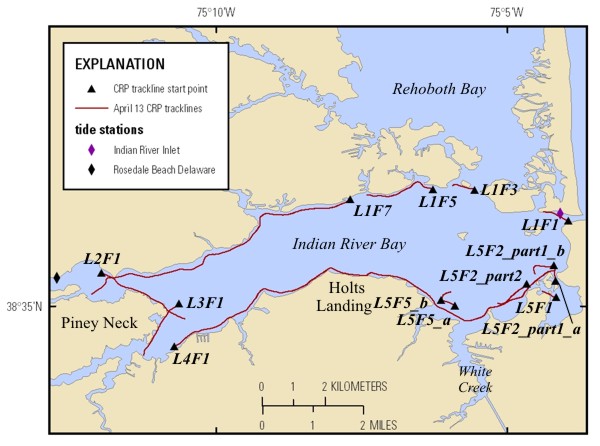
Continuous Resistivity Profile Previews - April 13, 2010The table below contains previews of the CRP data processed using average measured water resistivity values. Two of the lines on this day were additionally processed using a water conductivity file (file extension CON) that provides continuous, varying water resistivity values along the length of the lines. These lines (L1F7 and L4F1) extend almost the whole length of the bay from the inlet (more saline water) to Piney Neck (fresher water). Both the EarthImager 2D JPEG image and the MATLAB JPEG image of each processed file are presented. In addition, the trackline map below is a “clickable” map. By clicking on a line name, a new window will open with the processed images from that particular line segment. This new window will contain the MATLAB JPEG image as well as a reduced version of the EarthImager 2D JPEG image (short version). In the cases of L1F7 and L4F1, the link is to the images of the profiles processed with the water conductivity file. The beginning of each line is marked with a triangle on the map. The left side of the associated JPEG image represents the beginning of the line and corresponds to the triangle on the map. April 13, 2010, corresponds to Julian day 103. |
|
 |
|
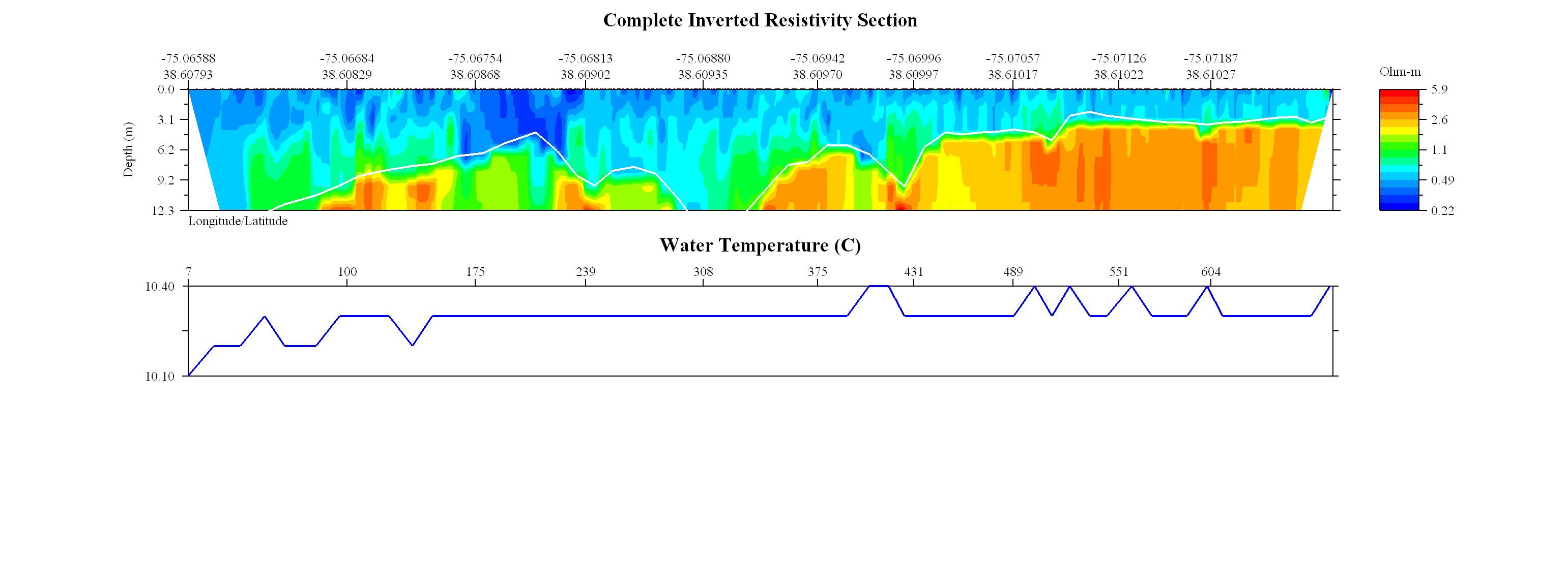
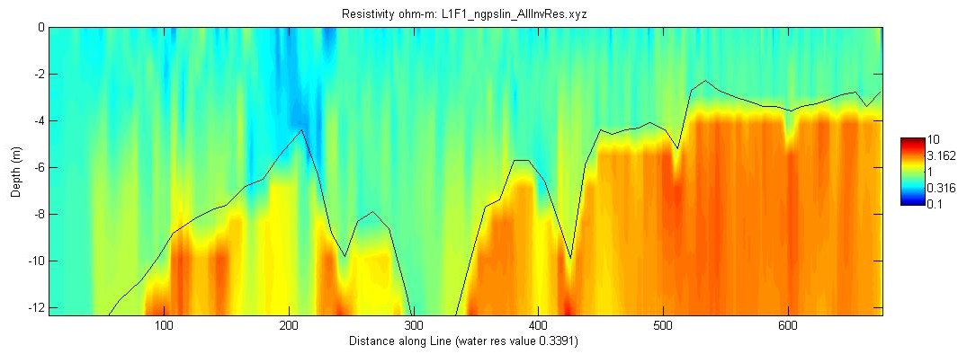
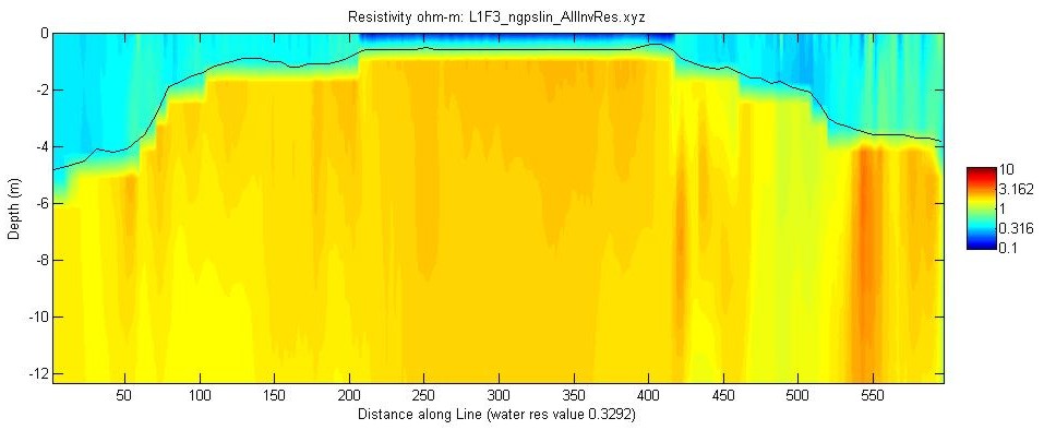
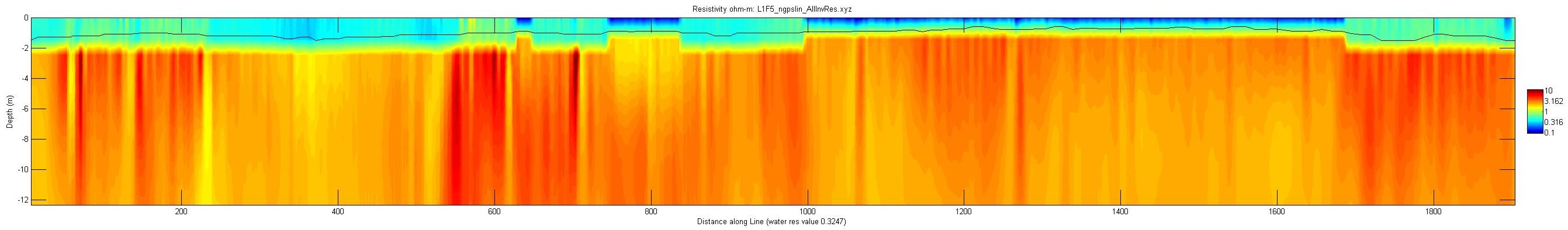
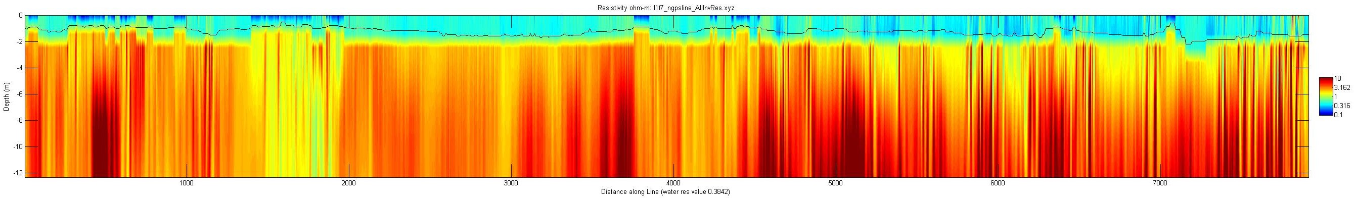
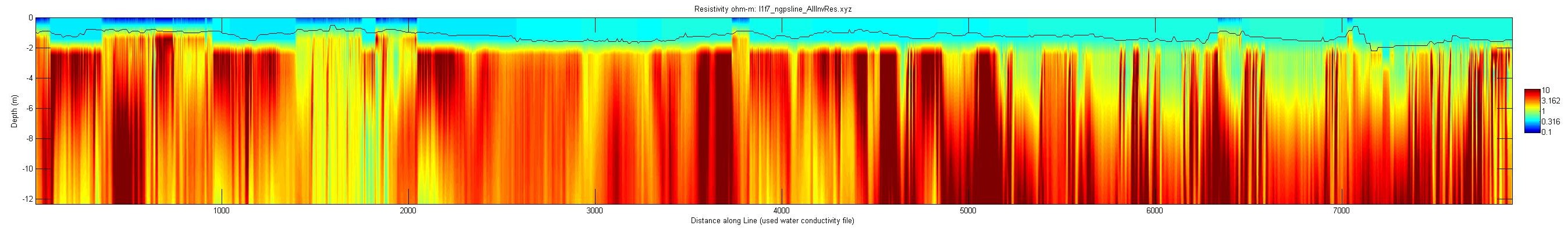
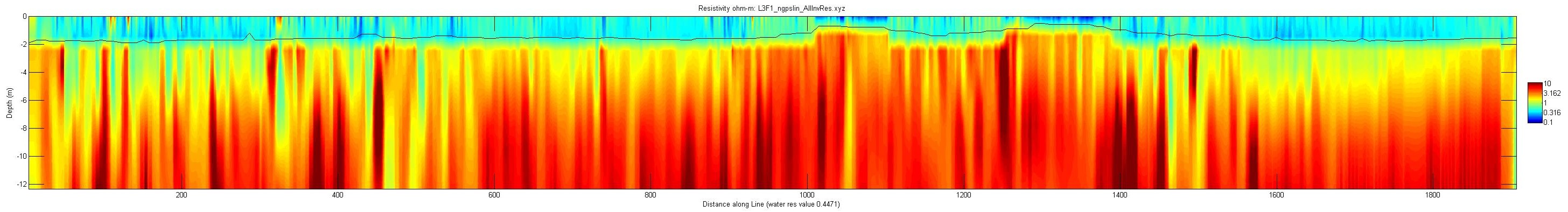
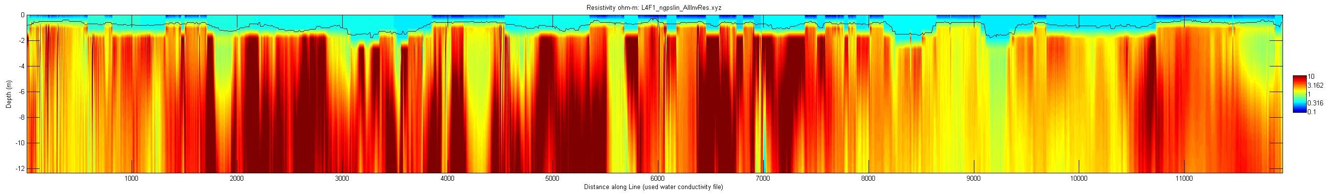
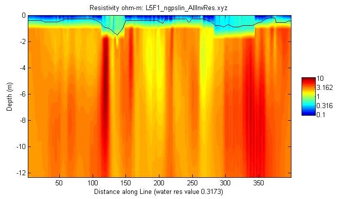
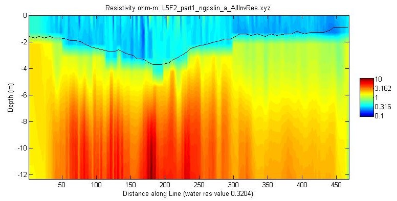
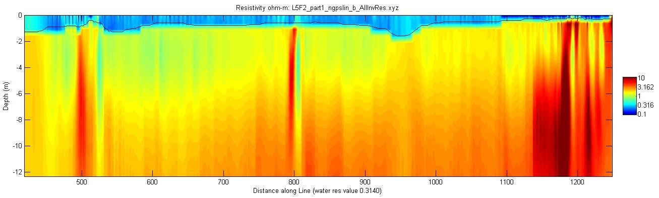
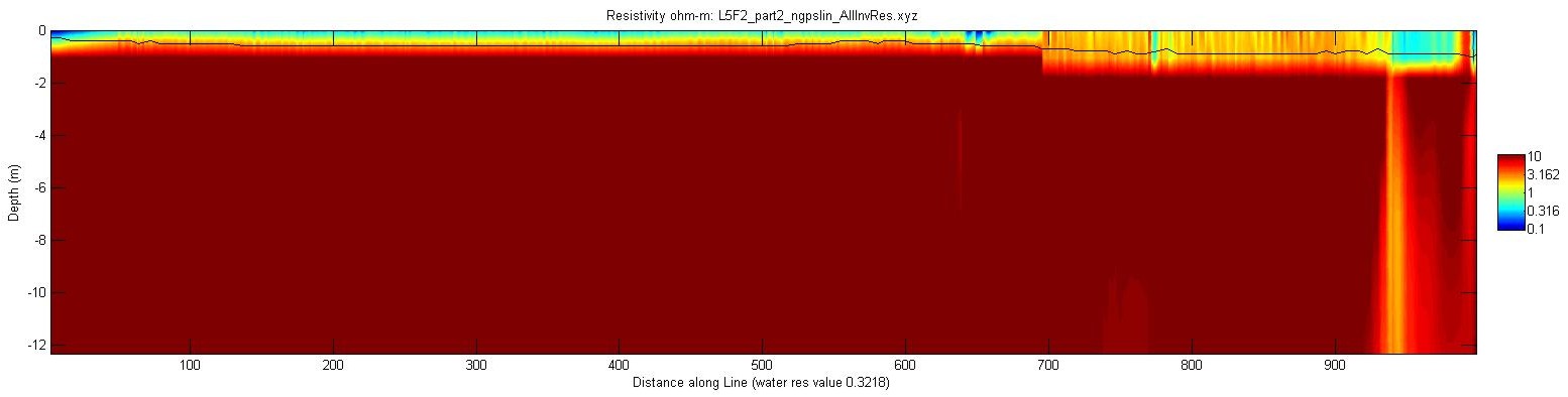
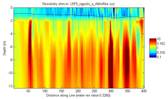
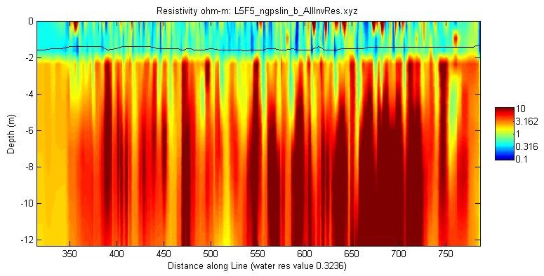
Preview of Profiles—Click individual images to see full-size JPEG images of the profile. For the EarthImager 2D versions, the long version of the profile is available. All of the profiles are available for download from the Data Catalog page In the EarthImager 2D version, the white line in the image represents the water depth as measured by the fathometer. In the MATLAB-generated JPEG images, the water depth is represented by a black line. The JPEG images resulting from the EarthImager 2D processing were saved with the default color scale generated by the software. This color scale ranges from blues to reds with reds representing the high resistivity values corresponding to fresher (less saline) groundwater. Each individual image has the scale maximized for the range of resistivity values in the dataset. The MATLAB versions of the JPEG images use a common color scale for all the files to facilitate profile comparison. For these images, the polarity of the color scheme is the same as that of the EarthImager 2D JPEGS in that the colors range from blue to red with reds indicating high resistivity values corresponding to fresher (less saline) groundwater. In the MATLAB version, the x axis represents distance along the line in meters. The EarthImager 2D version x-axis units are latitude and longitude (position) along the line. Measured water temperature information is included with the resistivity profile. |
|
| EarthImager version | MATLAB version |
|---|---|
April 13, 2010: Line L1F1, WRES = 0.3391 |
 |
April 13, 2010: Line L1F3, WRES = 0.3292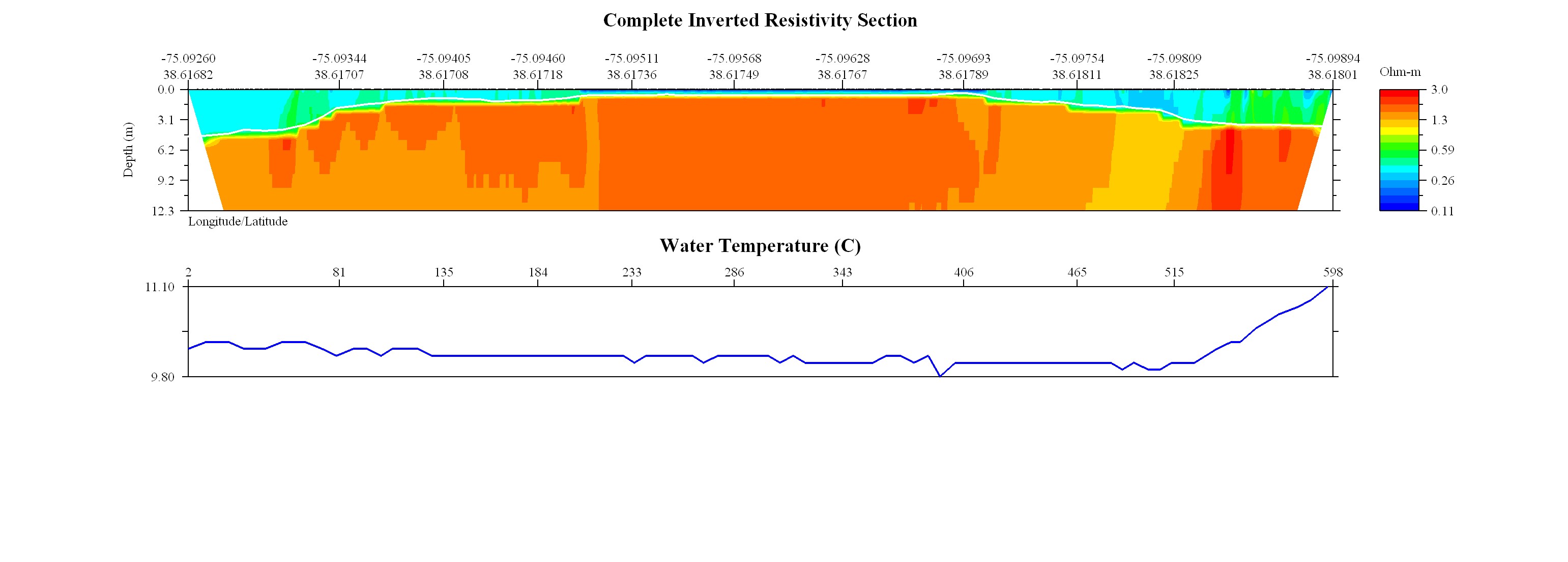 |
 |
April 13, 2010: Line L1F5, WRES = 0.3247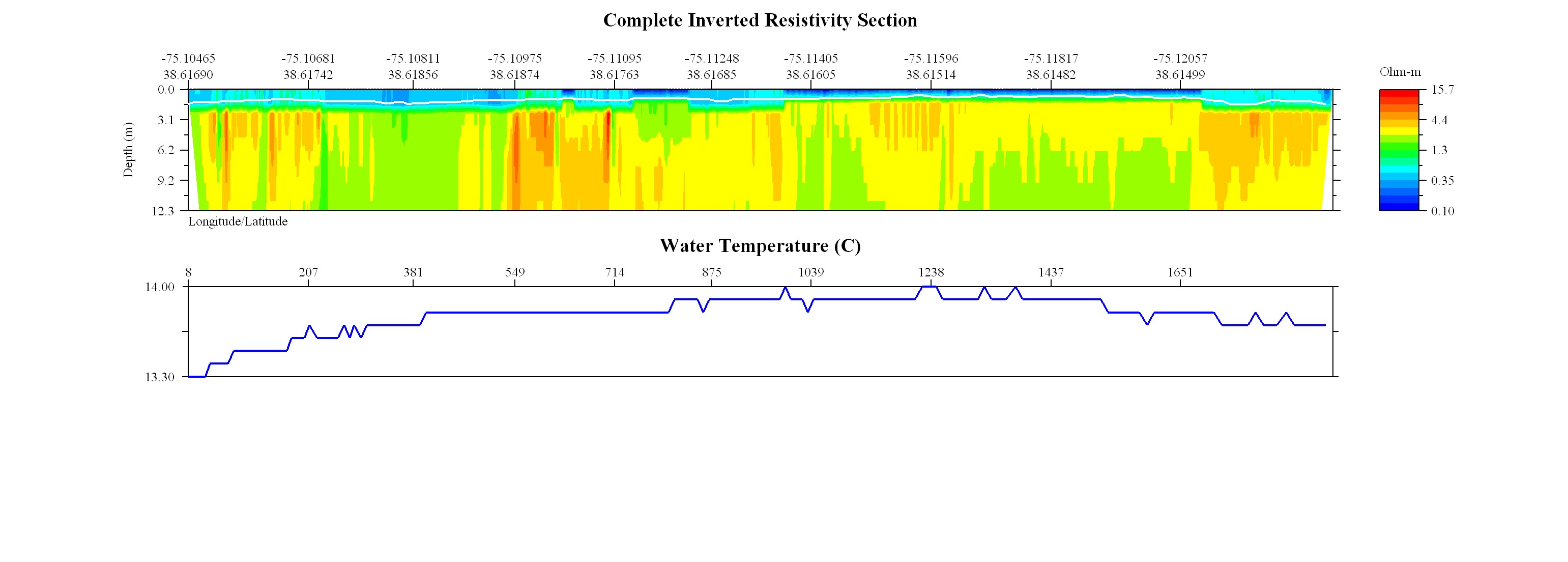 |
 |
April 13, 2010: Line L1F7, WRES = 0.3842 |
 |
April 13, 2010: Line L1F7, water conductivity file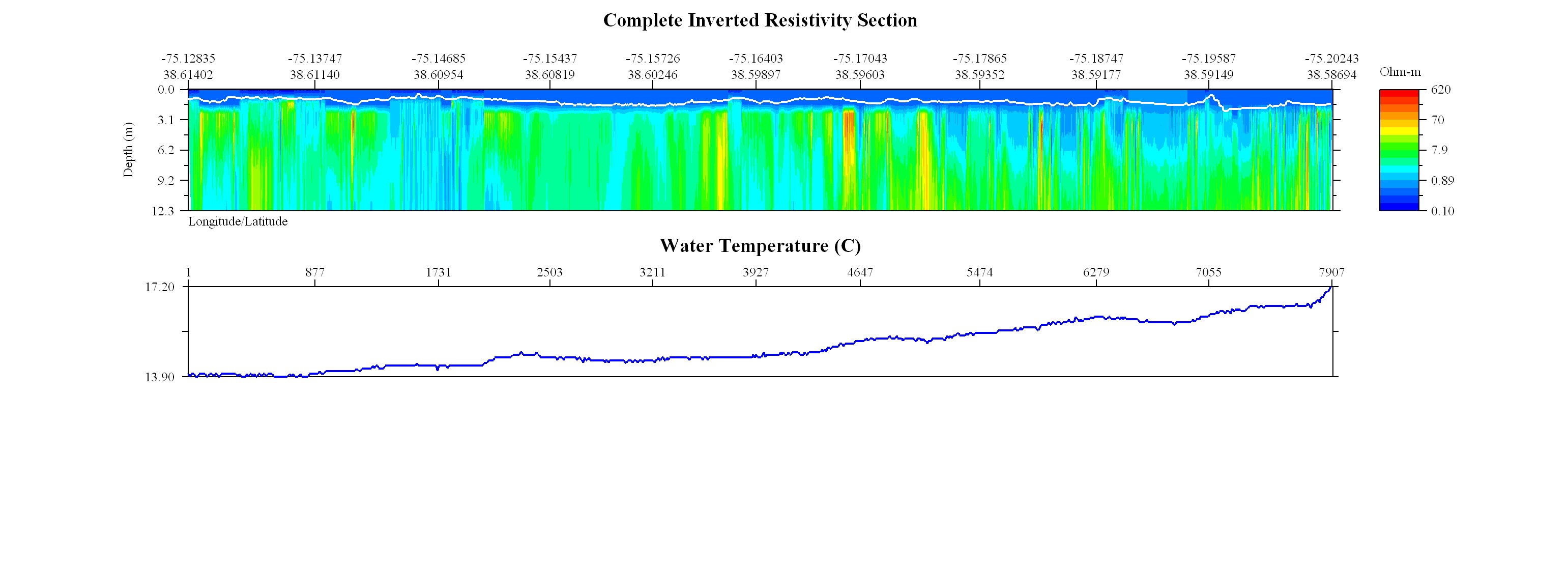 |
 |
April 13, 2010: Line L2F1, WRES = 0.4137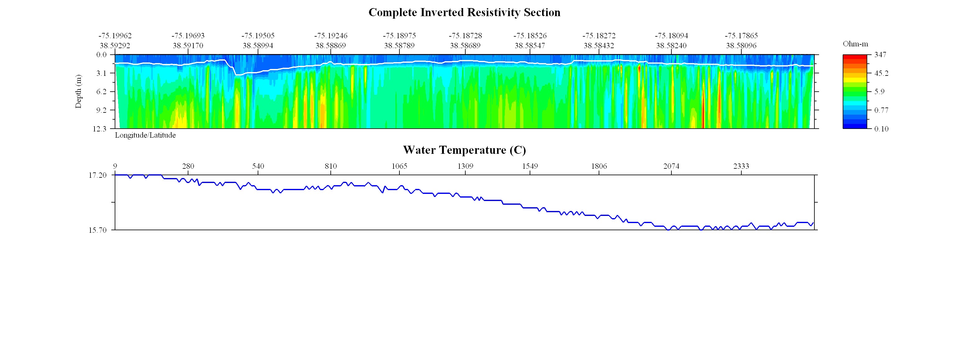 |
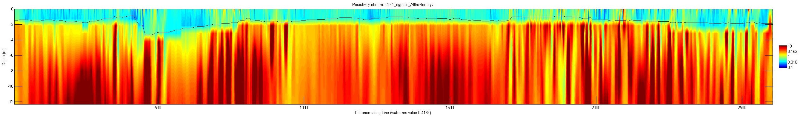 |
April 13, 2010: Line L3F1, WRES = 0.29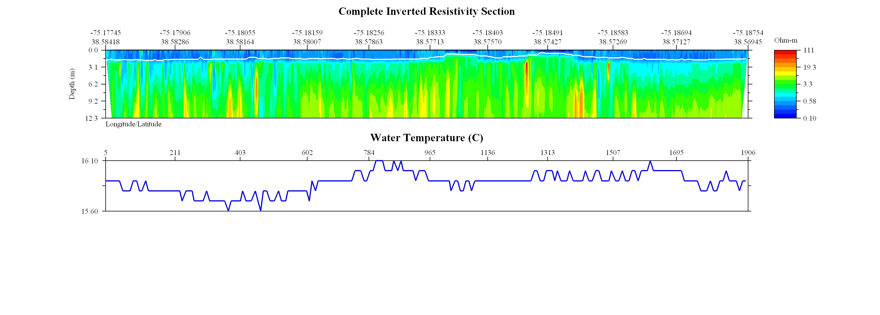 |
 |
April 13, 2010: Line L4F1, WRES = 0.3594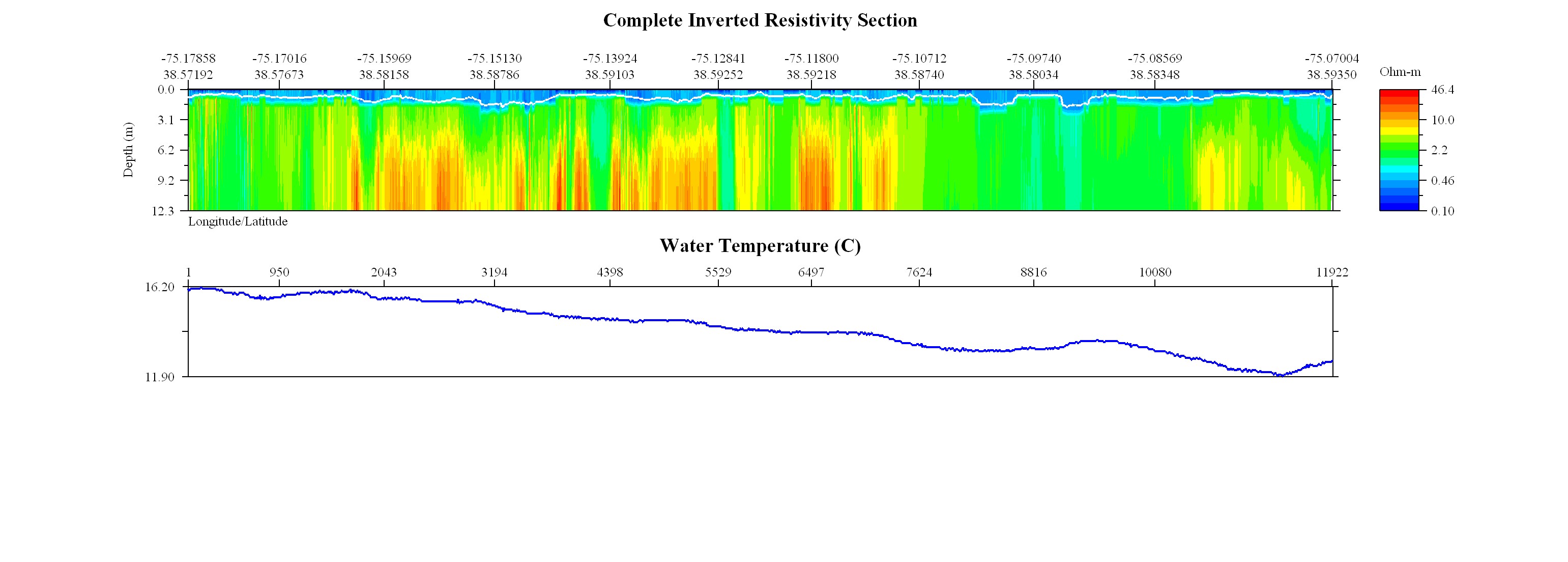 |
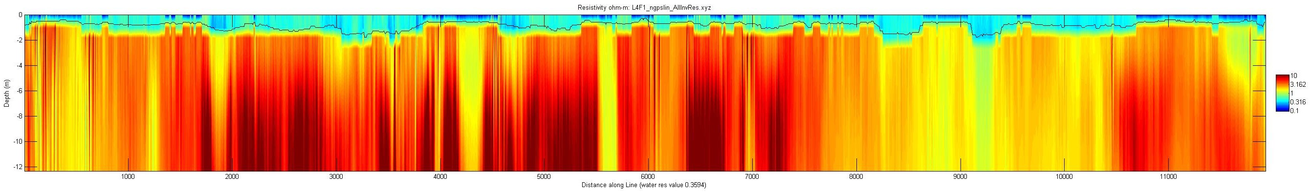 |
April 13, 2010: Line L4F1, water conductivity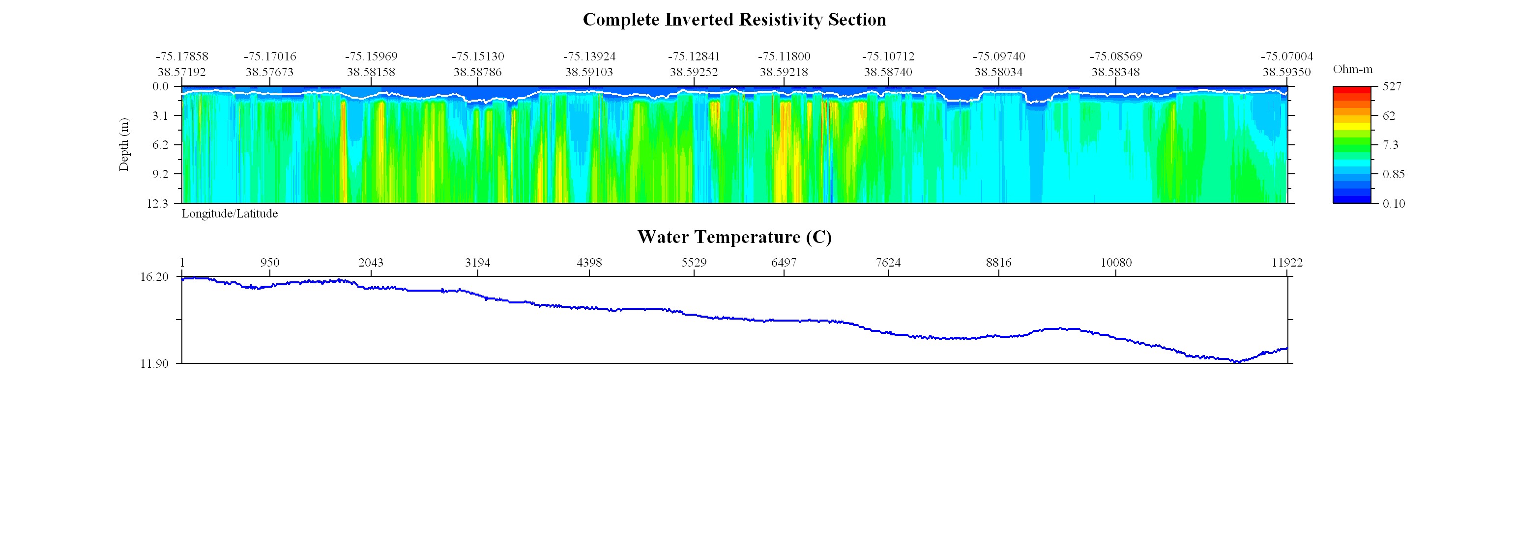 |
 |
April 13, 2010: Line L5F1, WRES = 0.3173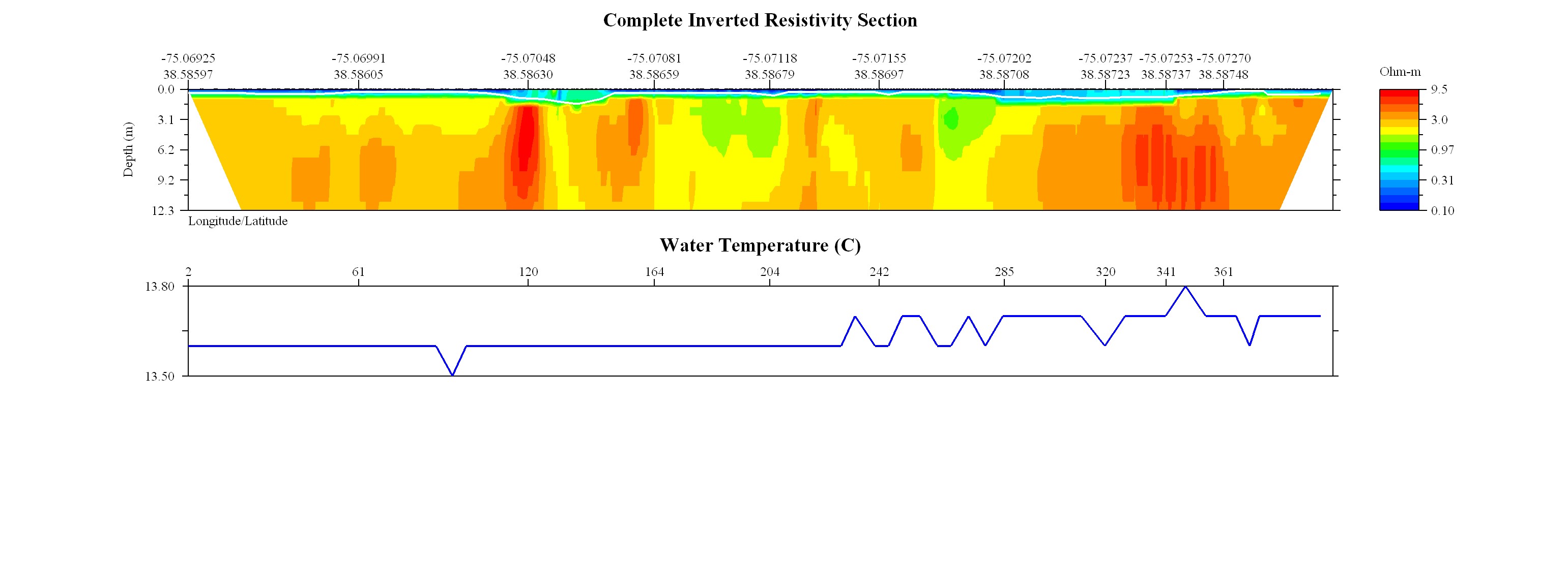 |
 |
April 13, 2010: Line L5F2_part1_a, WRES = 0.3204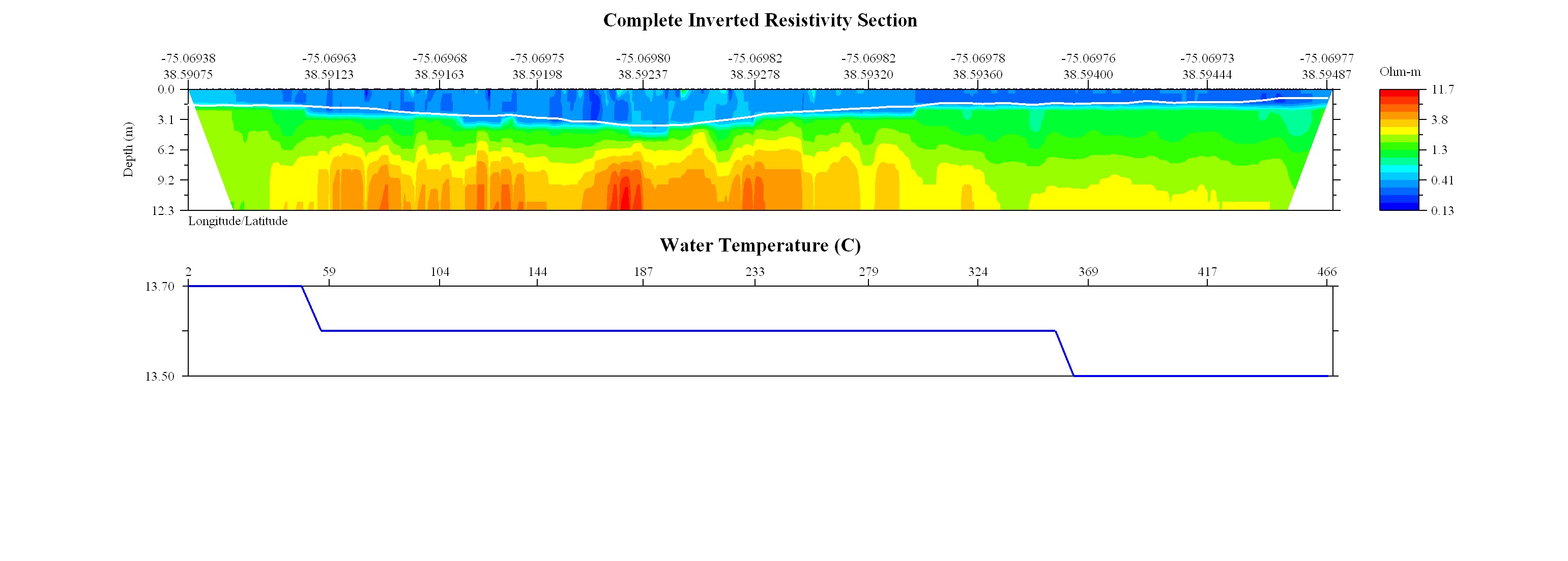 |
 |
April 13, 2010: Line L5F2_part1_b, WRES = 0.3140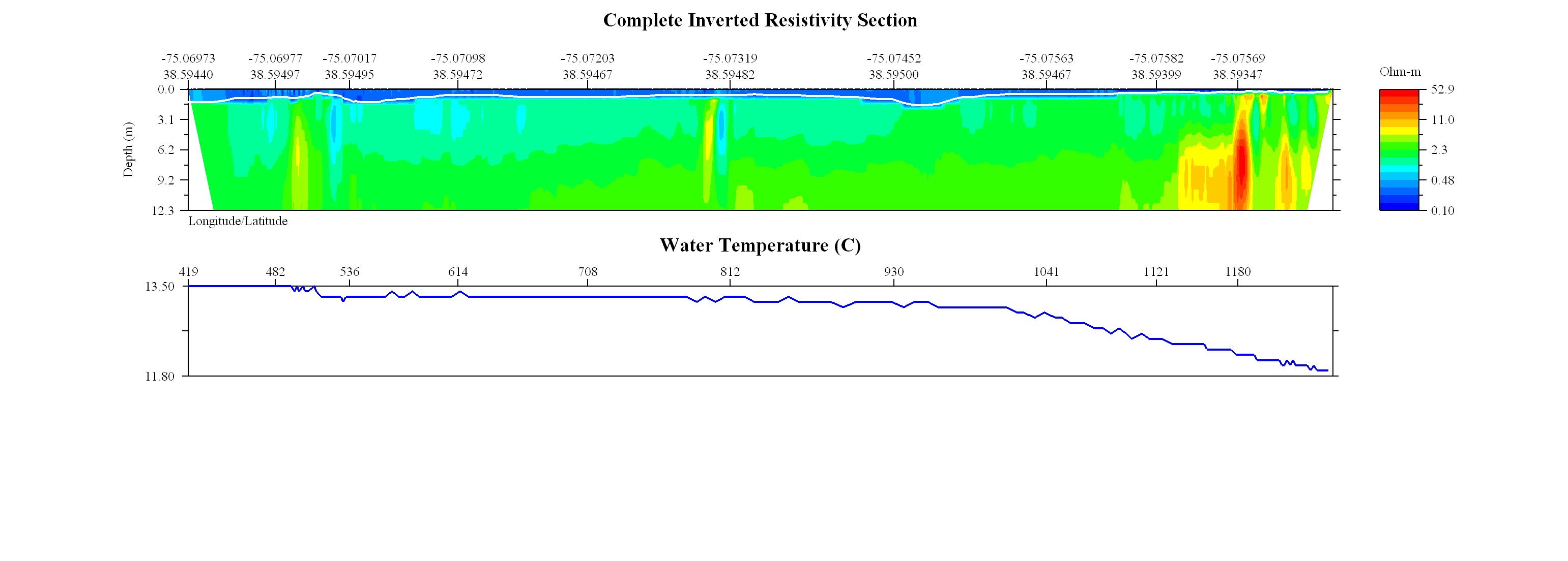 |
 |
April 13, 2010: Line L5F2_part2, WRES = 0.3218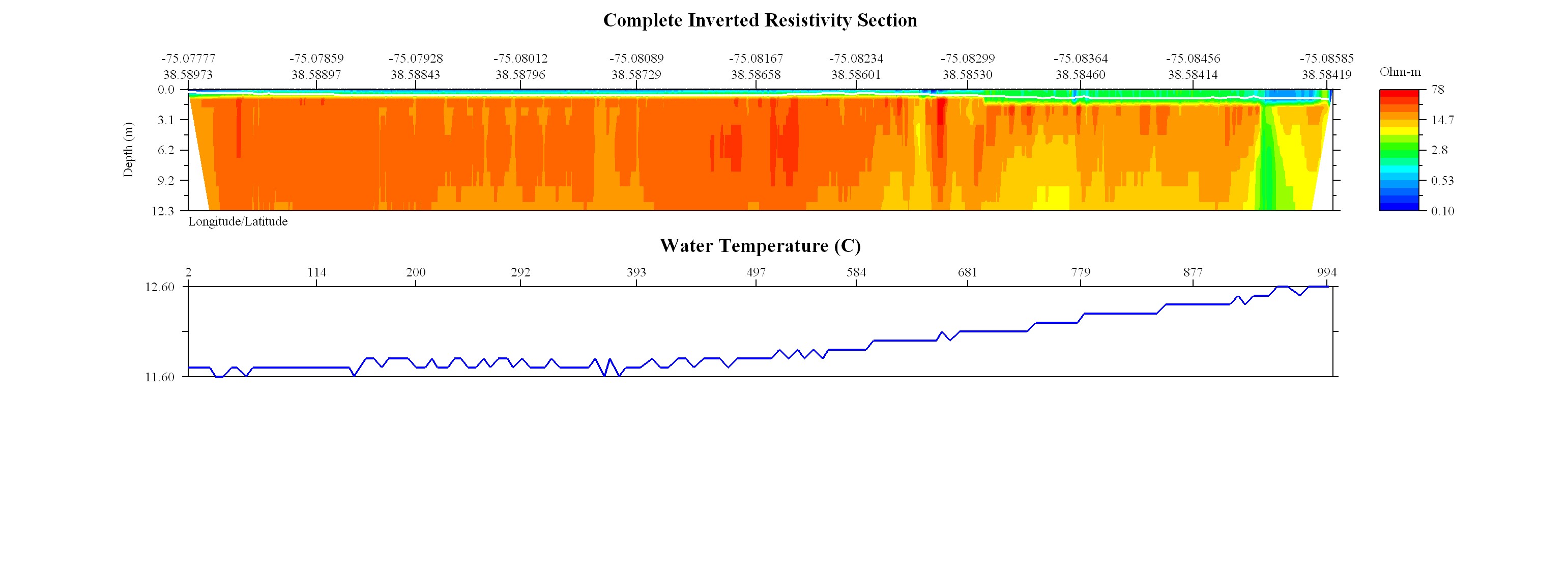 |
 |
April 13, 2010: Line L5F5_a, WRES = 0.3260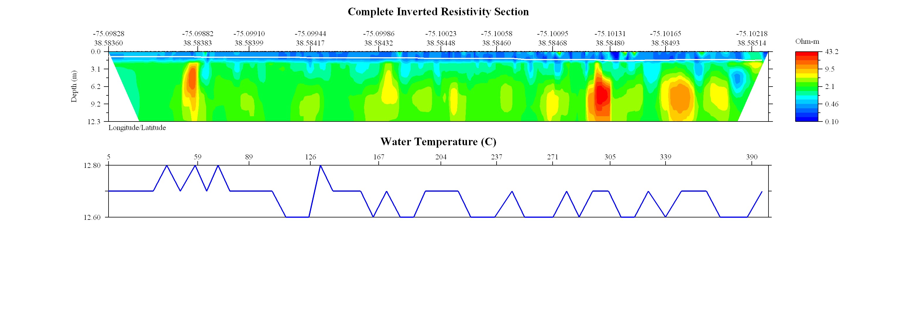 |
 |
April 13, 2010: Line L5F5_b, WRES = 0.3236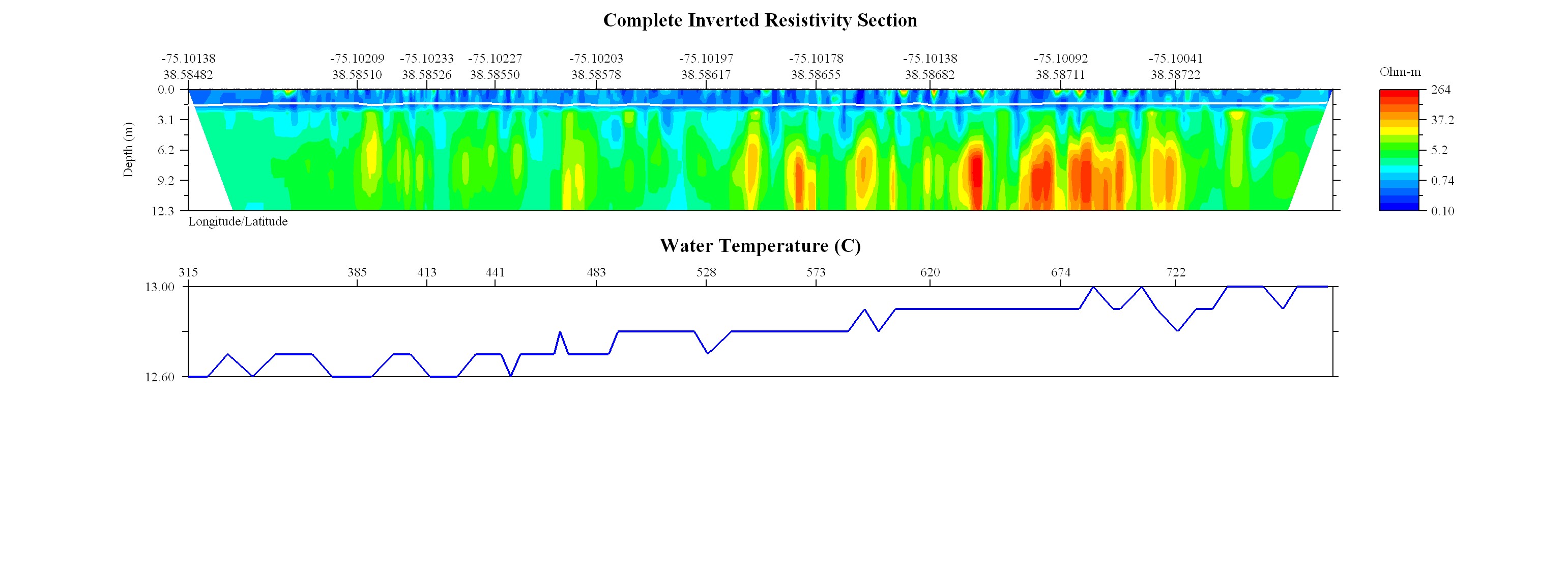 |
 |

![]() U.S. Department of the Interior |
U.S. Geological Survey
U.S. Department of the Interior |
U.S. Geological Survey
URL: http://pubsdata.usgs.gov/pubs/of/2011/1039/html/ofr2011-1039-resistprev_apr13.html
Page Contact Information: GS Pubs Web Contact
Page Last Modified: Thursday, 24-Jul-2014 14:14:01 EDT