Click on figures for larger images.

Figure 1. OSAT3 model domain within A, the northern Gulf of Mexico and B, showing bathymetry. Colors in B represent water depths relative to the North American Vertical Datum of 1988 (NAVD88). Analysis of model results extends from Dauphin Island, Ala., to Panama City Inlet, Fla.

Figure 2. Schematization of wave height and direction observations from NDBC buoy 42040 for April 1, 2010, to August 1, 2012. Colors indicate the percentage (%) of the occurrence for each wave height-direction bin. Wave height bins (numbered H1–H5) are organized from the center outward with larger waves (2 m and higher) in the outer ring (H5). Wave direction bins (numbered D1–D16) each span 22.5 degrees (°), from 0° to 360°, labeled around the circumference of the diagram.

Figure 3. Generation of alongshore currents due to wave breaking at an angle to the Gulf coast of Alabama and Florida. Image used with permission (COMET®) Website, 2011).

Figure 4. A, Modeled wave height from the H5_D7 scenario simulation (fig. 2; wave height more than 2 m from the southeast); B, associated wave-driven current vectors showing resolution of the cross-shore variable alongshore current profile (arrow length is proportional to current speed). The number of current vectors has been reduced by a factor of six in the cross-shore direction in B for better viewing. Color gradation near the coast in B illustrates depth-induced wave breaking in shallow water depths.

Figure 5. Elevations (NAVD88) at three levels of detail for Little Lagoon Inlet, Ala. A, 30–m resolution digital elevations (Love and others, 2012); B, 1-m resolution lidar elevations (USACE, 2010); and C, fall 2012 2-m resolution stereoanalysis elevations (Aero-Metric, Inc., unpub. data, 2012). A gradational scale of elevations and depths is provided to illustrate the increased resolution at the inlet.

Figure 6. Distribution of surface residual ball (SRB) density (ρ) calculated from chemical composition along the Alabama and Florida Gulf coast. Data are from L. Bruce, British Petroleum Corporation, GCRO, Science/NRDA Team (unpub. data, 2012).

Figure 7. Processes driving surface residual ball (SRB) and sediment mobility and transport along the Alabama and Florida Gulf coast. Wave- and current-induced shear stress can resuspend sand, SRBs, and other material from the sea floor, leading to potential transport by currents. (Symbols used by permission from Integration and Application Network, 2012).

Figure 8. Critical shear stress (in Pa) of surface residual balls (SRBs) along the Alabama and Florida Gulf coast as a function of diameter (in cm). Shown are values calculated using the original Shields (1936) formulation, and a modified version accounting for exposure wherein the dimensionless sheer stress approaches a constant value for particles that are partially exposed (0.1) or fully exposed (0.2; see appendix 3).

Figure 9. Critical stress of sand and surface residual balls (SRBs) along the Alabama and Florida Gulf coast, after Shields (1936) shown as a function of density and grain size for six particle sizes. For each standardized surface residual ball (SRB) grain size (table 1), we calculate the critical stress for the range of observed SRB densities, with the resultant critical stress mean and one standard deviation shown. The critical stress calculated for each size using the mean SRB density is within the small range of variability but is greater than the critical stress of a particle of the same size with the density of quartz sand.

Figure 10. Two mechanisms of increased probability for surface residual ball (SRB) accumulation based on A, alongshore flow convergence and B, spatially decelerating flows.

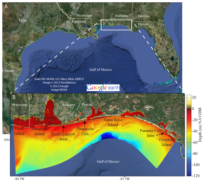
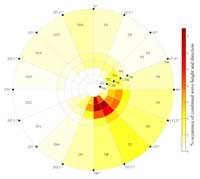
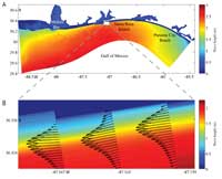
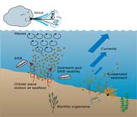
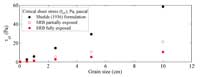
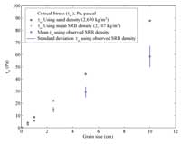
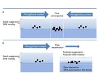
Modeling Approach

Hydrodynamic simulations included scenarios derived from wave and weather observations at the National Data Buoy Center (NDBC; 2012) buoy 42040 from April 1, 2010, to June 1, 2012. This buoy was just offshore of the eastern side of the OSAT3 model domain. The wave observations were schematized by dividing wave heights into 5 bins bounded by 0.0, 0.5, 1.0, 1.5, 2.0, and 5.0 m and sampling wave directions in 16 bins each spanning 22.5 degrees (°), from 0° to 360°. The combination of wave height and direction bins yielded 80 different scenarios. The probability of occurrence of each scenario (fig. 2) indicated that waves were most likely to have heights of 0.5 to 1.0 m and come from the southeast. However, the set of scenarios that were considered included common and relatively rare wave conditions. The details of selecting scenarios are described in appendix 1.

Due to the large geographic extent and variability of the model domain, application of spatially homogeneous wave conditions along the entire offshore model boundary would provide unrealistic results. Therefore, for each of the scenarios, the observed wave record was searched for a specific time that most closely matched the characteristics of the scenario. Then, archived results from the National Weather Service (NWS) National Center for Environmental Prediction (NCEP) NOAA Wavewatch III regional wave model (Environmental Modeling Center, 2012), corresponding to that specific time, were applied to the OSAT3 model domain boundaries. Archived winds from the same regional model, also corresponding to the same point in time, were applied to the free-surface boundary of the entire OSAT3 model domain. Stationary wave conditions were used and variations in water level were not considered for the scenario simulations.

In addition to the stationary scenarios, two time periods were simulated to evaluate model accuracy over a range of conditions: (1) January 15–25, 2007, which included both quiescent and storm conditions during winter and (2) Hurricane Isaac on August 27–31, 2012, an extreme weather event during summer. For these simulations, time-varying wave conditions were imposed on the boundaries of the OSAT3 model.

Hydrodynamic Model Description

We used the Delft3D (version 4.00.01) coupled wave-flow model to compute stirring associated with wave orbital velocities and steady wave and wind-driven alongshore currents (Lesser and others, 2004; Deltares, 2007). The model computes flow variables using the depth-averaged shallow water equations that are intrinsically relevant to analyzing alongshore currents in the domain, particularly in the surf zone. We used model parameter values that have been demonstrated in Lesser and others (2004) to be appropriate for the sandy coastlines similar to those within our project area. Model parameters are documented in appendix 2 as part of the example input files for the Flow and Wave modules.

Three-dimensional surf zone processes were not simulated due to the focus on the prediction and role of alongshore currents (as opposed to cross-shore processes) in transporting SRBs along the project domain. In the nearshore environment, currents are caused primarily by wave-breaking processes. Reniers and others (2004) showed that vertical profiles of wave-driven alongshore currents are relatively depth-uniform, indicating that the use of depth-averaged models is acceptable. Density stratification was also assumed to be negligible due to intense vertical mixing by breaking waves and stratification was not included in the model equations. Winds are included in the model to generate waves within the domain. Although currents caused by wave breaking processes are dominant in the nearshore environment, the model also simulates currents generated by wind blowing over the ocean surface. Variable water depth and its influence on wave refraction, shoaling, and breaking and alongshore current magnitude and location was included.

Alongshore current directions and magnitudes (for example, eastward or westward following the curvature of the model grid) were required to understand the movement of sediments and SRBs under various wave conditions. Waves approaching the shoreline at an angle break and transfer their momentum to the water column, creating the primary force that is responsible for driving alongshore currents (fig. 3). Generally, waves approaching from the west drive currents to the east and vice versa. Depending on the local geometry of the coast and nearshore bathymetry, complex spatial patterns in the magnitude and direction of the alongshore current can develop. The cross shore and alongshore variations of the nearshore currents were resolved with the model grid and depict the alongshore current jet that is driven by wave breaking near the shoreline (fig. 4).

Hydrodynamic Model Input Data

Bathymetry

Bathymetric data (fig. 1) were obtained from the northern Gulf Coast digital elevation map of the NOAA National Geophysical Data Center (NGDC; Love and others, 2012). These data, with 30-m resolution, satisfied the large-scale needs of the OSAT3 domain. An exception was at Little Lagoon Inlet, Ala., which, at 10 m wide, required higher grid resolution and more accurate bathymetric data (fig. 5A) to define the inlet for simulations, including tidal variations. Refined inlet resolution was not used in the scenario simulations where temporal water level variations were not considered. At Little Lagoon, we used data from the U.S. Army Corps of Engineers (USACE, 2010) collected in January through March 2010, just before the Deepwater Horizon oil spill (fig. 5B). Additionally, for the Little Lagoon Inlet, we assimilated stereoelevation data collected as part of the spill response (Aero-Metric, Inc., unpub. data, 2012) to improve simulation results, determine the sensitivity of modeled flows to bathymetric changes, and demonstrate an ability to integrate this relatively novel data source (fig. 5C).

Geomorphic features larger than the smallest grid cells of the model (that is, 250 m in the alongshore and 10 m in the cross-shore) were resolved in the model. Thus, nearshore features such as sandbars, mega cusps, and other features relevant to this effort were evaluated. These nearshore features, however, are highly ephemeral, and temporal variations were not resolved over the approximately 2-year time period that the simulations represented. Lidar or stereometric observations (fig. 5B, C) near Little Lagoon represented more recent and accurate snapshots of bathymetric variation. Large offshore features such as submarine canyons that can affect the wave climate were spatially resolved by the models providing boundary conditions to the domain use in our modeling simulations.

Waves

Archived results from the NOAA Wavewatch III operational 4-minute ('), or about 7.5-kilometer (km)-resolution U.S. East Coast and Gulf of Mexico wave model (Tolman, 2008; Environmental Modeling Center, 2012) were used for the boundary conditions in the Wave module of Delft3D. This wave model is part of a nested series of operational models of varying sizes and resolutions that extend to a global-scale parent grid. The model system has been run, essentially in the stated configuration, since February 2005, and NOAA provides archives of bulk wave parameters at 3-hour intervals from modeled hindcasts. Wave heights, periods, and directions from Wavewatch III were extracted and prescribed along the offshore and lateral boundaries of the OSAT3 domain with an assumed Joint North Sea Wave Project (JONSWAP) spectral shape (Hasselmann and others, 1973). The boundary conditions were prescribed at every thirtieth grid cell, matching the coarse resolution of the Wavewatch III model. Wave conditions for the scenario simulations were held stationary. For the time series simulations, wave conditions were updated every 3 hours. The directional domain for the wave model covered a full circle with a resolution of 5° (72 bins in total), and the frequency domain was 0.05 to 1 hertz (Hz) with logarithmic spacing. The bottom-friction dissipation parameterization of Hasselmann and others (1973) was used with a uniform bottom roughness coefficient of 0.067 square meters per second cubed (m²/s³). Additionally, so-called third-generation physics were activated, accounting for wind wave generation, triad wave interactions, and white capping by the Komen and others (1984) parameterization. Depth-induced wave breaking dissipation was included using the Battjes and Janssen (1978) parameterization with default values for alpha (1) and gamma (0.73). More details regarding input parameters can be found in the Wave input file in appendix 2.

Winds

Wind velocities were also obtained from the archived Wavewatch III 4'-resolution data. NOAA uses winds from their Global Forecast System weather model to generate waves in Wavewatch III and stores this wind data in the Wavewatch III archives (Environmental Modeling Center, 2012). These wind velocities were extracted from the archives and applied over the entire OSAT3 model domain. As done for the waves, the wind velocities for the scenario simulations were held stationary whereas for the time series simulations wind velocities were updated every 3 hours.

Tides and Surge

Variations in water levels were accounted for in the time-series simulations. Water levels imposed at the model boundaries were obtained from the TPXO7.2 global tide model which uses a numerical tidal model and satellite-derived observations of tide elevation to produce tidal constituents (Egbert and Erofeeva, 2010). Subtidal water level fluctuations that accounted for regional oceanographic processes were obtained from a large-scale ocean model (Hybrid Coordinate Ocean Model, 2012a) that simulated tides and surge within the Gulf of Mexico with a resolution of approximately 4 km. Hybrid Coordinate Ocean Model (HYCOM; 2012b) data assimilation incorporates observations of water level derived from satellite altimeters, which increases prediction accuracy. Hourly water level variations from the combination of tidal and subtidal water level models were imposed at the two offshore corners of the domain and linearly interpolated along the offshore boundary. Spatially varying tidal flows into and out of the inlets and estuaries along the project site were included and evaluated in time series simulations.

SRB and Sand Movement

The goal of assessing SRB response to hydrodynamic conditions is split into determining the likelihood of SRBs to move (thresholds for incipient motion, for example, mobility, are exceeded), the likelihood to be buried or exhumed by surrounding sediment, the propensity for alongshore transport, and the tendency to accumulate. SRB burial and exhumation are more likely in areas of more mobile sediment, particularly where sand is mobile and SRBs are immobile. The types of analysis conducted for each scenario and time-series, therefore, were SRB mobility, local surficial sediment mobility, and SRB potential flux, which was used as a proxy to identify probable alongshore patterns in SRB redistribution. The exact velocity and alongshore transport distances of individual SRBs could not be assessed because the locations of SRBs or their sources are unknown. We are also limited by some fundamental uncertainties about SRB transport (see Discussion section).

Physical Properties of Sand and SRBs

The response of sand and SRBs to hydrodynamic forces is a function of the size and density of the particles. For sediment (without oil), the median grain size in the surf zone in this region was determined to vary between 0.250 and 0.500 millimeters (mm; D.C. Phelps and others, Florida Geological Survey, unpub. data, 2011). Sand in this region was predominantly quartz (Balsam and Beeson, 2003) and therefore of approximately 2,650-kilogram per cubic meter (kg/m3) density. Quantitative information on SRB chemical composition came from an OSAT-supplied dataset (L. Bruce, British Petroleum Corporation, Gulf Coast Restoration Organization (GCRO), Science Natural Resource Damage Assessment Team (NRDA), unpub. data, 2012) and was used to calculate the variability in density (fig. 6; appendix 3). Observational data on the size distribution of SRBs were not available, therefore a range of classes (0.03 centimeters (cm), 0.5 cm, 1 cm, 2.5 cm, 5 cm, and 10 cm) were chosen to span the estimated range of SRB size variability (W. Bryant, U.S. Geological Survey, oral commun., 2012).

Physical Processes of Sand and SRBs

The processes that were considered in the SRB and sediment mobility and transport analysis included stirring due to wave orbital motion at the sea floor, alongshore currents, and tidal currents at inlets (fig. 7). SRBs or sand grains will begin to move when the shear stress force associated with the combined action of waves and currents exceeds a size- and density-specific critical threshold value. See appendix 3 for calculation of shear stress from hydrodynamic results and calculation of critical stress thresholds. Localized turbulence and wave-to-wave variation can cause any individual particle to move at calculated stress values below threshold; however, the formulations used here, on average, have been found to be accurate for surf zone calculation (Deigaard and others, 1991; Soulsby and others, 1993).

Critical stress values could also be affected by particle shape and exposure above the sea floor. The empirical mobility relationship originally developed by Shields (1936) and used in this analysis is for a uniform bed of well-packed sediment, and larger particles such as SRBs extruding above the bed would have a lower critical value for mobility than estimated with the standard Shields calculation (Fenton and Abbott, 1977; Andrews, 1983; Wiberg and Smith, 1987; Wilcock, 1998; Bottacin-Busolin and others, 2008). Because individual SRBs may have varying exposure above the surrounding sea floor, three critical stress values were considered to account for departures from the simple assumption in Shields (1936). The high critical stress values recorded during the study would be the ones required to move unexposed SRBs sitting approximately level with the surrounding bed, such as might be expected in a recently fragmented mat. The medium critical stress values correspond to a partially exposed SRB, and the low critical stress values correspond to a single isolated SRB fully exposed atop on the sea floor (appendix 3). The medium and low critical stress values for any given particle are roughly a third and a sixth of the high critical stress estimate (fig. 8). Local surficial sediment mobility was assessed using a single critical stress value based on the Shields parameterization or the high estimate for SRBs because the sand in the northern Gulf of Mexico surf zone is of generally uniform size.

Sand and SRB Representative Class Definition

To estimate the mobility and potential flux associated with the modeled waves and currents, SRB or local sediment diameter and density must be specified. Particle density is well constrained for the predominantly quartz sand in this region but varied somewhat for observed SRBs. The sensitivity of the critical stress required for inducing particle mobility was examined for a range of densities consistent with SRB data. The variations in SRB density caused relatively small critical stress variations compared with the differences due to variations in SRB size and in comparison sand mobility (fig. 9). Thus, particle diameter was the dominant control on mobility (figs. 8 and 9). Therefore, overall SRB variability was characterized by a set of six classes of varying size and fixed density. Local sediment was characterized by a single size and density (table 1).

Inlet Dynamics and Sediment Mobility

The influence of tidal currents on sediment transport, including sand and SRBs, in the vicinity of tidal inlets and estuaries is more complicated than the open-coast analysis where wave-generated alongshore currents dominate flow patterns. Inlet effects caused by tidal flows and their interaction with the incoming wave field (wave-current interaction) were evaluated across the model domain for 24 hours using wind and wave parameters of scenario H4_D7 (fig. 2). Identifying inlet convergence and divergence patterns requires detailed shallow bathymetry at the inlet. The model grid used for inlet simulations at Pensacola Pass, Fla., Little Lagoon, and Panama City (fig. 1) therefore included higher (for example, 1- to 50-m) alongshore resolution within the three inlets. The flow field and water levels were coupled with the wave model every 3 hours to include the effects of flow and water level processes on the incoming waves for simulations of sediment mobility at inlets.

Metrics for Evaluating Sand and SRB Mobility and Redistribution Patterns

Analyses were conducted to determine sediment and SRB movement probability and alongshore redistribution patterns for SRBs of size classes for each individual scenario, illustrating the likely mobility and redistribution patterns under the conditions that scenario represents. In addition, metrics of mobility and alongshore potential flux were calculated as weighted averages of all the scenarios, indicating probable patterns in mobility and redistribution over longer time scales, and mobility over a 24-hour period was calculated for one scenario to assess the variability in mobility over a tidal cycle.

Metrics for hydrodynamic and SRB and sediment movement probability and alongshore redistribution for wave scenarios are:

• significant wave height;
• maximum and median alongshore current;
• alongshore current convergences;
• alongshore current decelerations;
• mobility ratio; and,
• potential flux.

Two additional metrics used to assess the overall probability of mobility and alongshore distribution over the time period of interest are:

• weighted mobility probability; and,
• weighted potential flux.

The range of tidally induced SRB and sand mobility over a 24-hour period for one scenario is evaluated with:

• tidal mobility.

These metrics are listed in table 2 with the naming convention of the associated output shapefiles (appendix 4). Metric calculations are described below.

Significant Wave Height

The significant wave height (metric 1) is calculated by the Wave module of Delft3D for each scenario. This parameter is an output of the model, is converted to Esri ArcGIS polygon shapefile format over the model domain, and is included to illustrate the spatial variability in wave height for each scenario.

Maximum and Median Alongshore Current

The alongshore component of the flow velocity within the surf zone was extracted from each scenario simulation (for example, see fig. 4). The modeled surf zone for each scenario was defined as stretching from the shoreline out to the cross-shore location of maximum wave height found between the shoreline and the most offshore point of modeled, depth-induced wave breaking dissipation. The maximum and median surf zone alongshore current at each alongshore location, for each scenario, was extracted within this surf zone (metric 2). The currents (maximum and median) were smoothed over a 2-km alongshore region to remove short-scale, noisy variations associated with grid-scale variations that were not well resolved.

Alongshore Current Convergences

The alongshore varying maximum velocity computed above was used to identify flow convergences (metric 3) and decelerations in the magnitude of flow in the direction of flow movement, indicating locations where the alongshore transport of SRBs would be disrupted and deposition would be more likely (fig. 10). Locations of convergences in the maximum alongshore current were computed by finding adjacent grid cells where the current velocity transitioned from eastward-directed (positive alongshore velocity) to westward-directed (negative alongshore velocity). The convergence is always selected as the negative (westward) velocity cell.

Alongshore Current Decelerations

Spatial decelerations in the direction of flow (metric 4; for example, the flow velocity decreases from one grid cell to the adjacent cell in the direction of flow) were defined using an advective acceleration term, δu/δy, where u is the alongshore current and y is the alongshore grid coordinate. The derivative of u was computed and used to identify locations where the flow decelerated (δu/δy less than (<) 0). We identified locations corresponding to peak deceleration (convex points in δu/δy) and the magnitude of u δu/δy at the identified points was also recorded. Note that, for eastward flow (u greater than (>) 0), the u δu/δy deceleration term is negative, whereas for westward flow (u < 0), the u δu/δy deceleration term is positive.

Sand and SRB Mobility Ratio

Sand and SRB mobility (metric 5) was assessed by calculating the ratio of the spatially variant maximum combined wave-current bed shear stress (τ_WC) for each scenario (appendix 3) to the three critical stress values for each representative SRB class. A mobility ratio greater than one indicated critical stress value exceedance and, therefore, particle mobility. Also calculated was the mobility ratio of the local sand-sized sediment. When sand is mobilized, there is the potential for SRB exhumation or burial. The magnitude of the mobility does not indicate distance, direction, or velocity of transport. Movement may consist of rocking back and forth in wave action with no net motion or net cross-shore transport.

SRB Surf-Zone Integrated Alongshore Potential Flux

To assess alongshore transport patterns, the approach of Soulsby-van Rijn (Soulsby, 1997) was used to develop estimates of SRB combined suspended and bedload potential flux. The Soulsby-van Rijn method accounts for currents, which are the dominant force in alongshore transport, and waves, which contribute a stirring action that keeps particles in motion and allows them to move with current velocities otherwise too weak to support transport. The potential flux was calculated as the mass per second that would be transported across a meter span in the cross-shore. To estimate the total alongshore flux at each alongshore location, the potential flux (in kilograms per meter per second) in each grid cell was multiplied by the cross-shore width of that grid cell to attain the total rate of mass passing through the cell (in kilograms per second). Results from each grid cell in the surf zone at each alongshore location were then added together to attain the total potential rate of mass transfer (in kilograms per second), resulting in an integrated potential flux alongshore the surf-zone (metric 6). The alongshore variant potential flux for each scenario was smoothed with a sliding 2-km Hanning window (Bendat and Piersal, 1971) to remove smaller scale spatial variation not likely to be well resolved by the model.

The Soulsby-van Rijn formulation was developed to estimate flux for a uniform bed of particles of a given size. The actual flux in the case of a mixed bed, such as SRBs mixed in with sand, will be a function of the relative availability of each material. If no SRBs are present, then the flux for the materials in the bed will be 0. The spatial patterns in the potential flux, however, highlight areas where there are flux convergences and (or) zones of decreasing flux magnitude in the direction of flow, both of which would be more probable areas for SRB deposition. Conversely, flux divergences and (or) zones of increasing flux magnitude in the direction of flow are less likely to accumulate SRBs. The flux sensitivity to the three critical stress values described above (fig. 8) was considered in order to account for potential variability due to exposure above the sea floor.

Weighted Mobility Probability

In addition to individual scenario results, the results from multiple scenarios were combined to assess persistent patterns in mobility during April 1, 2010, to August 1, 2012. For each scenario, the mobility map was converted to a binary threshold map delineating locations where the critical value for mobility had been exceeded (value = 1) and not exceeded (value = 0). For sand and each SRB class and critical threshold value, an average of this threshold exceedance map was taken, weighted by the scenario probability of occurrence over the 2-year time period considered (appendix 1). The weighted mobility probability (metric 7) varies from 0 to 1, with values approaching 1 indicating mobility under most wave conditions and values approaching 0 indicating little to no mobility under any wave conditions. The weighted mobility probability is a measure of the probability that SRBs or sand are mobilized and is analogous to the fraction of time at each location that mobility occurred over the time period of interest, whereas the mobility ratio for an individual scenario as previously described, which can be any number greater than or equal to 0, is the ratio of the stress to the critical threshold value for the single point in time represented by that scenario and must exceed 1 to indicate mobility under the conditions of the scenario.

Weighted Potential Flux

In addition to the potential flux for each individual scenario, an average surf-zone integrated potential alongshore flux (smoothed over 2 km in the alongshore direction) was calculated for each SRB class and critical stress threshold from all the scenarios, weighted by scenario probability (metric 8). This analysis shows patterns in SRB redistribution over all wave conditions during the 2-year period considered and may thus highlight persistent patterns in SRB alongshore redistribution, assuming that cross-shore processes did not transport SRBs and remove them from the surf zone (either through onshore deposition or loss to the shelf) between individual events.

Tidal Mobility

The tidal-inlet simulation produces a measure of tidally induced SRB and sand mobility near inlets, referred to as tidal mobility (metric 9). The simulation is based in part on metric 5 (table 2), the mobility ratio, and calculated hourly over a 24-hour tide cycle for scenario H4_D7. The results are output in polygon shapefile format for each of the 24-hour time steps. Appendix 5 includes the time step and shapefile (TT) corresponding to maximum flood and ebb for each inlet in the model domain, and file naming conventions are defined in appendix 4.

Tidal Inlet Animations

In addition to tidal mobility metrics (table 2) assessed over the entire model domain for each size class of SRB and sand, animated movies (.avi file format) of the mobility of 2.5-cm SRBs and sand were created to demonstrate the temporal variation in mobility over the tidal cycle for Pensacola Pass, Fla., Little Lagoon, Ala., and Panama City, Fla. (fig. 1). See appendix 4 for file naming conventions.