Click on figures for larger images.

Figure 11. NDBC directional wave buoys (42012, 42039, and 42040) and a Naval Research Laboratory (NRL) acoustic doppler current profiler (ADCP) used for model evaluation along the Alabama and Florida Gulf coast.

Figure 12. Comparison of Wavewatch III and SWAN model output to significant wave height and wave period observations at NDBC buoy 42012 between May 1, 2010, and May 1, 2011.

Figure 13. Model predictions of A, wave height and B, wave direction from the 80 scenarios compared with observations at NDBC buoy 42012 in the northern Gulf of Mexico alongshore Alabama and Florida. Shown are scenarios when mean offshore wave direction (buoy 42040) was from the southeast, south, and southwest (wave direction bins D5–D12; fig. 2) and from northwest, north, and northeast (wave direction bins D1–D4 and D13–D16; fig. 2). The error statistics correspond to modeled waves for D5–D12 scenarios.

Figure 14. Model predictions of A, wave height (H), B, peak wave direction (Dp), and C, peak wave period (Tp) in the northern Gulf of Mexico alongshore Alabama and Florida for January 15–25, 2007, compared with observations (wavecis) from a Naval Research Laboratory acoustic doppler current profiler at Santa Rosa Island, Florida. To demonstrate the accuracy of the model, we show the values from NDBC buoy 42040 offshore in the northern Gulf of Mexico as an alternative model for predicting nearshore values. Only cases where the measured nearshore wave height exceeded 0.5 meter are shown.

Figure 15. Evaluation of accuracy of simulated (modeled) water levels (in meters) against NOAA tidal measurements at A, three coastal inlet tide stations at B, Dauphin Island, Ala., C, Pensacola Pass, Fla., and D, Panama City Inlet, Fla. Astronomical water level predictions are also shown. The model predictions include some noise in the initial spinup of the flow simulations, which disappears after a few tidal cycles.

Figure 16. Simulated and measured wave characteristics at buoy 42012 (fig. 11) in the northern Gulf of Mexico alongshore Alabama and Florida during Hurricane Isaac in August 2012. Characteristics include A, significant wave height, B, mean wave direction, and C, mean wave period.

Figure 17. Simulation of water levels (in meters) in the northern Gulf of Mexico alongshore Alabama and Florida during Hurricane Isaac in August 2012 compared with measured water level at the NOAA tide stations at A, Dauphin Island, Ala., B, Pensacola, Fla., and C, Panama City, Fla. tide stations (fig. 15A) and to astronomical tide predictions.

Figure 18. Significant wave height (table 2, metric 1) for scenarios A, H3_D6 and B, H3_D8 (fig. 2) in the northern Gulf of Mexico alongshore Alabama and Florida. Nearshore wave height in each scenario originated with 1- to 1.5-meter (m)-high waves at National Oceanic and Atmospheric Administration buoy 42040, but with southeasterly and south-southeasterly wind directions, respectively.

Figure 19. Maximum alongshore velocity (table 2, metric 2) smoothed over a 2-kilometer length scale for scenarios A, H3_D6 and B, H3_D8 (fig. 2) in the northern Gulf of Mexico alongshore Alabama and Florida. Green and red arrows indicate eastward- and westward-directed flows, respectively. Flow is to the west throughout the domain in A, whereas there are mixed flow directions in B.

Figure 20. Flow convergence (table 2, metric 3) for scenarios A, H3_D6 and B, H3_D8 (fig. 2) in the northern Gulf of Mexico alongshore Alabama and Florida. Flow reversals are absent in A, whereas several flow reversals were identified in B and correspond to color changes in fig. 19B.

Figure 21. Flow deceleration (table 2, metric 4; as change, delta, d, meters per second squared, m/s2) for scenarios A, H3_D6 and B, H3_D8 (fig. 2) in the northern Gulf of Mexico alongshore Alabama and Florida. Spatial decelerations of varying magnitudes are found in both scenarios.

Figure 22. Mobility ratio (table 2, metric 5) in the northern Gulf of Mexico alongshore Alabama and Florida for a midlevel threshold of 2.5-centimeter surface residual balls (SRBs; table 1) for scenarios A, H3_D6 and B, H4_D6 (fig. 2). Areas with a mobility ratio of 1 (in pink) indicate where the mobility threshold was exceeded. Whereas the mobility threshold is exceeded only in small sections in very shallow water in A, the large wave heights result in mobility along the coast as well as over shallow bar and ebb tidal delta features in B .

Figure 23. Mobility ratio (table 2, metric 5) in the northern Gulf of Mexico alongshore Alabama and Florida for sand for scenarios A, H3_D6 and B, H4_D6 (fig. 2). Areas with a mobility ratio of 1 (in pink) indicate where the mobility threshold was exceeded. Compared with 2.5-centimeter surface residual balls (SRBs; fig. 22), sand is mobile over a large portion of the domain in both scenarios, yielding the potential for exhumation and burial of SRBs in regions where the SRBs themselves are immobile.

Figure 24. Mobility ratio (table 2, metric 5) in the northern Gulf of Mexico alongshore Alabama and Florida for a midlevel threshold of 2.5-centimeter (cm) surface residual balls (SRBs; table 1) along the Gulf Islands National Seashore (east of Pensacola Pass, Florida) for wave scenario H5_D1, corresponding to waves observed at NDBC buoy 42040 of height greater than 2 meters and coming from a north-northeasterly direction (fig. 2). Where the mobility ratio exceeded 1 (in pink) mobility of 2.5-cm SRBs was indicated at locations along the back-barrier from northerly wind-waves locally generated behind the barrier.

Figure 25. Surf-zone integrated alongshore potential flux smoothed over 2 kilometers (table 2, metric 6) for 2.5-centimeter surface residual balls (SRBs; table 1) in the northern Gulf of Mexico alongshore Alabama and Florida for scenarios A, H3_D6 and B, H4_D6. Because of the limited mobility in A (fig. 23), there is virtually no potential flux, whereas there is westward potential flux throughout the domain in B. Areas where the magnitude of the flow decreases (B, inset) are more likely areas of SRB deposition.

Figure 26. Weighted mobility probability (table 2, metric 7) from April 2010 to August 2012 along the Gulf Islands National Seashore (east of Pensacola Pass, Fla.) for 2.5-centimeter surface residual balls (SRBs). Shown is an estimate using A, the highest estimate of critical stress, appropriate for SRBs flush with the seabed, and B, the lowest estimate of critical stress, appropriate for SRBs sitting atop the seabed.

Figure 27. Weighted surf-zone integrated alongshore potential flux (table 2, metric 8), indicating the average potential flux in the northern Gulf of Mexico alongshore Alabama and Florida from April 2010 to August 2012 for 2.5-centimeter surface residual balls (SRBs; table 1) using a midrange estimate of critical stress. There is a convergence in the probable flux at Pensacola Pass, Fla., and divergence toward the east of Pensacola Pass.

Figure 28. Tidal inlet surface residual ball (SRB) mobility (table 2, metric 9) at A, maximum flood and B, maximum ebb for 2.5-centimeter SRBs (table 1) using a low critical threshold at Little Lagoon Inlet, Ala. (fig. 1). Areas where the mobility ratio is 1 (in pink) indicate that the critical threshold for SRB mobility is exceeded. The greater extent of tidal inlet SRB mobility during flood increases the probability that SRBs brought in by the tide will remain trapped. Local surficial sediment is mobilized throughout the illustrated domain during both flood and ebb tide, leading to potential for burial and exposure of SRBs.

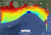
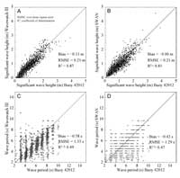
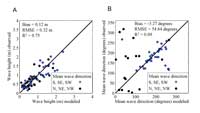
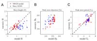
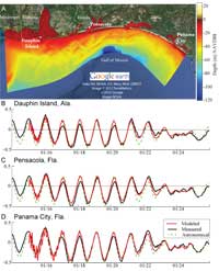
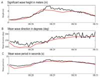
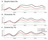
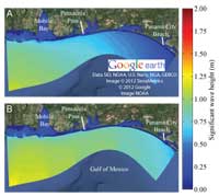
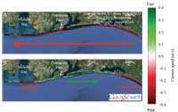
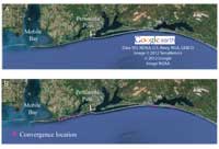
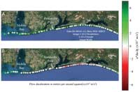
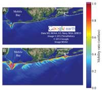
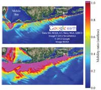
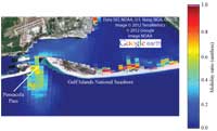
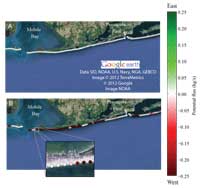
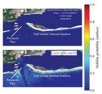
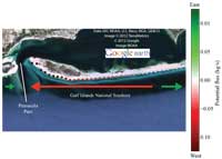
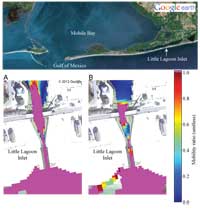
Model Evalulation

Wave Model

NDBC directional wave buoy, 42012, (National Data Buoy Center, 2012) off the coast near the Florida-Alabama border, is in 28-m water depth and lies within the OSAT3 model domain (fig. 11). In addition, a wave-resolving acoustic doppler current profiler (ADCP) had been deployed in the project area. We used the observations from the ADCP to evaluate the accuracy of the wave model and to evaluate the suitability of the large-scale wave model to providing boundary conditions for the high-resolution model (K.T. Holland, Naval Research Laboratory, unpub. data, 2012). We evaluated the sensitivity of large-scale model predictions to changes in model resolution at the boundary using the Wavewatch III model results. The output of Wavewatch III 4'-resolution between May 2010 and May 2011 was compared with a validated, high resolution (2', or about 3.7-km) Simulating Waves Nearshore (SWAN; Booij and others, 1999; Ris and others, 1999) wave hindcast that was run by the USGS Woods Hole Coastal and Marine Science Center and to data from NDBC buoys in the northern Gulf of Mexico (National Data Buoy Center, 2012; fig. 11) over the longer time period of May 2010 to May 2012. Output from the closest grid cell to each buoy was used for model validation. Results from Wavewatch III and SWAN was comparable to data from three NDBC buoys (42012, 42039, and 42040). Specifically, at all three buoys the difference in bias (that is, mean) and root-mean-square (RMS) error in wave height (in meters) and period (in seconds) between the models was less than 0.2 m (fig. 12; table 3). The overall bias and RMS error, respectively, for the 2-year period were –0.10 m and 0.20 m for significant wave height and –0.56 s and 1.28 s for wave period at buoy 42012, the closest buoy to the project site. A similar magnitude of error was obtained at two more offshore northern Gulf of Mexico buoys (table 4). This analysis demonstrates that the Wavewatch III model resolves wave conditions sufficiently to provide boundary conditions for the OSAT3 domain, and that accuracy would not be improved by running a higher resolution model to provide boundary conditions.

Timeseries of simulated wave conditions were extracted from the 80 simulation scenarios by comparing the observed wave height and direction at buoy 42040 to the scenario definitions and selecting the best-fit scenario for each hour. Then, simulated wave conditions at each hour were compared to observations from buoy 42012 (fig. 13). This evaluation demonstrates the modeled wave transformation from the offshore boundary to the interior of the OSAT3 model domain. Wave height was predicted well at this location, whereas directions were predicted well for offshore waves propagating at a mean direction from the south, southeast, and southwest, but poorly for waves from the north. We note that northern waves observed at the offshore buoy (42040) and buoy 42012 in about 30-m water depth usually correspond to small wave events along the coast of the northern Gulf of Mexico, which result in weak alongshore currents and therefore weak mobility or transport. These events also have a low probability of occurrence.

Finally, wave model predictions at Santa Rosa Island, Fla., for the winter time series (January 15–25, 2007) were compared with data collected by researchers at the Naval Research Laboratory (K.T. Holland, Naval Research Laboratory, unpub. data, 2012) for the same time period by an ADCP in approximately 12-m water depth. The comparison (fig. 14) shows that wave height was predicted within acceptable tolerance (0.24-m bias error and 0.31-m RMS error). Models of wave direction and periods produced a 27° and –1-s, respectively, bias error and 14° and 1-s RMS error, respectively. Largest errors in wave period and direction corresponded to the lowest wave heights (less than 0.5 m); these errors would have little impact on alongshore current or mobility calculation errors. The modeled peak period compares well with the observed mean period (fig. 14A–C).

Tide and Storm Simulations

NOAA operates tide stations at Dauphin Island, Pensacola Bay, and Panama City (National Oceanic and Atmospheric Administration, 2012). Observations from the permanent tide stations were used to evaluate the accuracy of water level predictions along the coast and into the bays within the project site for time-series simulations. We evaluated the accuracy of the tidal model using data from the tide stations for the January 15–25, 2007, time-series simulation. The comparison indicates minimal errors in both phase and amplitude at all locations (fig. 15).

The approach and landfall of Hurricane Isaac in late August 2012 was used to evaluate simulation accuracy under more extreme weather conditions. Wave characteristics and water level predictions were compared with waves measured at buoy 42012 (National Data Bouy Center, 2012) and to water level at the three NOAA tidal stations (National Oceanic and Atmospheric Administration, 2012; fig. 15). Wave height during the peak of the storm was slightly underpredicted, but predictions for mean wave direction and period showed reasonable approximations (fig. 16). It is not unusual for wind models to incorrectly predict the intensity of tropical storms (Rogers and others, 2006) and therefore lead to errors in modeled wave heights. The water level predictions underestimated water level observations at all locations (fig. 17). Our simulations relied on the large-scale models for adequate boundary conditions. We experimented with several different large-scale models to supply water level boundary conditions for the OSAT3 domain and determined that none of the alternate models offered improved accuracy compared with the others. The results here use HYCOM for large-scale water level boundary conditions at the OSAT3 model boundaries. Errors between the model and observations may reflect errors in the large-scale model predictions that provided boundary conditions to our simulations or shortcomings in the model implementation. The predictions were substantially improved compared with a simple astronomical prediction and captured the relevant dynamics associated with Hurricane Isaac's approach and landfall to the west of the area of interest.

Scenario Simulation Results

Results of the modeling simulations were exported from the irregular model grid as point and polygon shapefiles and are available in the digital release of this report. Alongshore patterns in currents, mobility, and potential flux varied significantly among the 80 scenarios, depending on the wave height and angle of approach and the amount of alongshore variability in the incoming wave field; variability in mobility around the inlets was noted over a tidal cycle.

Scenario Analysis

Figures 18 through 21 illustrate hydrodynamic analyses (table 2, metrics 1 to 4) from two scenarios, H3_D6 and H3_D8 (fig. 2). The selected scenarios present an offshore wave height of 1 to 1.5 m but from slightly different wind directions, southeast and south-southeast, respectively. Significant wave height (metric 1) barely reaches 0.75 m near the coast with the southeast winds (scenario H3_D6; fig. 18A), but significant wave height exceeds 1m with the south-southeast winds (H3_D8; fig. 18B). Maximum alongshore velocity (metric 2) is westward under scenario H3_D6 (fig. 19A) and mixed east and west under scenario H3_D8 (fig. 19B). Flow convergence (metric 3; meters per second, m/s) is absent under scenario H3_D6 (fig. 20A) but occurs at several different locations in scenario H3_D8 with the south-southeast wind (fig. 20B). Flow deceleration (metric 4; meters per second squared, m/s²) of varying magnitude and direction occurred under both scenarios (fig. 21). For scenario H3_D8 (figs. 20B and 21B), a combination of south-southeast waves, offshore features, and orientation of the coast produced numerous flow decelerations and reversals. Under scenario H3_D6 (figs. 20A and 21A), numerous alongshore convergences and spatial decelerations can affect the potential accumulation, burial, and removal of SRBs. The scenarios, while similar in originating wave energy and only 40° different in offshore wave angle, indicate that the movement of SRBs caused by alongshore flows is dependent on the specific wave conditions (for example, a specific time period of interest) and, potentially, the sequence of wave conditions over time that may allow SRBs to be transported from one area of accumulation to another.

The potential for movement of SRBs was assessed by calculating the mobility as represented by the ratio (table 2, metric 5) of the τ_WC for each scenario to the critical stress of incipient motion for each representative SRB class, with a mobility greater than 1 indicating that the threshold for mobility was exceeded (SRB and sand mobility section). For the H3_D6 scenario shown in figure 22A, with offshore waves between 1 and 1.5 m, the mobility threshold of 2.5-cm SRBs is only exceeded at isolated patches in the surf zone. In contrast, when the waves come from the same direction but the wave height increases to between 1.5 and 2 m, the mobility threshold of 2.5-cm SRBs is exceeded in a narrow band along the coastline and over shallow bar features (fig. 22B). In comparison, sand is mobilized under a significantly larger portion of the domain for both scenarios (fig. 23), with an associated potential for SRB exhumation or burial. In the case of northerly wind and wave scenarios (H5_D1), significant mobility may be found in some locations along the bay side of barrier islands (fig. 24).

The surf-zone integrated potential alongshore SRB flux (smoothed over 2 km) for each scenario and SRB class was calculated as described in the Methods section (table 2, metric 6; kilograms per second, kg/s). High, medium, and low critical stress estimates were analyzed to quantify the uncertainty in the potential flux estimates due to SRB exposure above the sea floor. Values less than 0 indicate transport to the west, values greater than 0 indicate transport to the east, values equal to 0 indicate no potential transport. Because of the limited mobility in scenario H3_D6 (fig. 25A), the potential flux is virtually 0, whereas for H4_D6 (fig. 25B), there are areas of potential flux (table 2, metric 6) throughout the domain for the model. The potential flux may be used to estimate likely spatial patterns in SRB redistribution; for example, in the illustrated scenario, 2.5-cm SRBs are more likely to be deposited where the magnitude of the westward potential flux decreases (fig. 25B detail).

SRB and Sand Weighted Mobility Probability and Potential Flux

The weighted mobility probability for SRB class 4 (fig. 26), calculated as described in Methods (table 2, metric 7), varied from 0 to 1, with values approaching 1 indicating that the mobility threshold was likely to be exceeded under most wave conditions, and values approaching 0 indicating mobility was unlikely under most conditions. Weighted mobility, which is the probability of mobility threshold exceedance, is analogous to the fraction of time an SRB of this size class is mobile. The variability between high, medium, and low mobility estimates provide a measure of the uncertainty in SRB mobility due to uncertainty in the estimation of critical stress thresholds. Alongshore Alabama and Florida on the northern Gulf of Mexico, 2.5-cm SRBs that are flush to the bed (highest estimate of critical stress among samples analysed; fig. 26A) are rarely mobilized, whereas SRBs more exposed to the flow field (lowest estimate of critical stress; fig. 26B) have a probability of mobilization of 0.6, corresponding to mobility approximately 60 percent of the time.

The weighted surf-zone integrated potential flux (table 2, metric 8; kg/s) is a measure of the long-term patterns in probable SRB movement. There is a convergence in the weighted potential flux of 2.5-cm SRBs around Pensacola Pass, indicating SRBs of this size are likely to accumulate at this location (fig. 27).

Tidal-Inlet Time-Series Results

The analysis of SRB and sediment mobility over a 24-hour period illustrates variability as a result of the tidal cycle. The variation in SRB mobility that can occur between ebb and flood near a coastal inlet can potentially lead to increased probability of SRB deposition within the lagoon over the tidal cycle (table 2, metric 9; fig. 28). The variation over the tidal cycle in mobility of sand and 2.5-cm SRBs can also be observed in animations, which are included in the digital release of this report, for the inlets at Pensacola Pass, Little Lagoon, and Panama City.