 |
| Click on figures for larger images. |
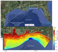 |
Figure 1. OSAT3 model domain within A, the northern Gulf of Mexico and B, showing bathymetry. Colors in B represent water depths relative to the North American Vertical Datum of 1988 (NAVD88). Analysis of model results extends from Dauphin Island, Ala., to Panama City Inlet, Fla. |
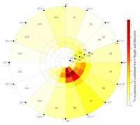 |
Figure 2. Schematization of wave height and direction observations from NDBC buoy 42040 for April 1, 2010, to August 1, 2012. Colors indicate the percentage (%) of the occurrence for each wave height-direction bin. Wave height bins (numbered H1H5) are organized from the center outward with larger waves (2 m and higher) in the outer ring (H5). Wave direction bins (numbered D1D16) each span 22.5 degrees (°), from 0° to 360°, labeled around the circumference of the diagram. |
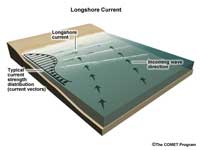 |
Figure 3. Generation of alongshore currents due to wave breaking at an angle to the Gulf coast of Alabama and Florida. Image used with permission (COMET®) Website, 2011). |
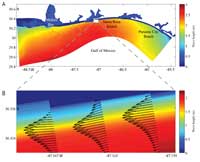 |
Figure 4. A, Modeled wave height from the H5_D7 scenario simulation (fig. 2; wave height more than 2 m from the southeast); B, associated wave-driven current vectors showing resolution of the cross-shore variable alongshore current profile (arrow length is proportional to current speed). The number of current vectors has been reduced by a factor of six in the cross-shore direction in B for better viewing. Color gradation near the coast in B illustrates depth-induced wave breaking in shallow water depths. |
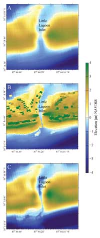 |
Figure 5. Elevations (NAVD88) at three levels of detail for Little Lagoon Inlet, Ala. A, 30m resolution digital elevations (Love and others, 2012); B, 1-m resolution lidar elevations (USACE, 2010); and C, fall 2012 2-m resolution stereoanalysis elevations (Aero-Metric, Inc., unpub. data, 2012). A gradational scale of elevations and depths is provided to illustrate the increased resolution at the inlet. |
 |
Figure 6. Distribution of surface residual ball (SRB) density (ρ) calculated from chemical composition along the Alabama and Florida Gulf coast. Data are from L. Bruce, British Petroleum Corporation, GCRO, Science/NRDA Team (unpub. data, 2012). |
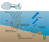 |
Figure 7. Processes driving surface residual ball (SRB) and sediment mobility and transport along the Alabama and Florida Gulf coast. Wave- and current-induced shear stress can resuspend sand, SRBs, and other material from the sea floor, leading to potential transport by currents. (Symbols used by permission from Integration and Application Network, 2012). |
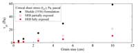 |
Figure 8. Critical shear stress (in Pa) of surface residual balls (SRBs) along the Alabama and Florida Gulf coast as a function of diameter (in cm). Shown are values calculated using the original Shields (1936) formulation, and a modified version accounting for exposure wherein the dimensionless sheer stress approaches a constant value for particles that are partially exposed (0.1) or fully exposed (0.2; see appendix 3). |
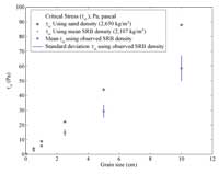 |
Figure 9. Critical stress of sand and surface residual balls (SRBs) along the Alabama and Florida Gulf coast, after Shields (1936) shown as a function of density and grain size for six particle sizes. For each standardized surface residual ball (SRB) grain size (table 1), we calculate the critical stress for the range of observed SRB densities, with the resultant critical stress mean and one standard deviation shown. The critical stress calculated for each size using the mean SRB density is within the small range of variability but is greater than the critical stress of a particle of the same size with the density of quartz sand. |
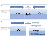 |
Figure 10. Two mechanisms of increased probability for surface residual ball (SRB) accumulation based on A, alongshore flow convergence and B, spatially decelerating flows. |
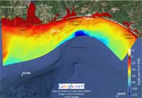 |
Figure 11. NDBC directional wave buoys (42012, 42039, and 42040) and a Naval Research Laboratory (NRL) acoustic doppler current profiler (ADCP) used for model evaluation along the Alabama and Florida Gulf coast. |
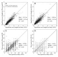 |
Figure 12. Comparison of Wavewatch III and SWAN model output to significant wave height and wave period observations at NDBC buoy 42012 between May 1, 2010, and May 1, 2011. |
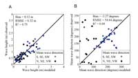 |
Figure 13. Model predictions of A, wave height and B, wave direction from the 80 scenarios compared with observations at NDBC buoy 42012 in the northern Gulf of Mexico alongshore Alabama and Florida. Shown are scenarios when mean offshore wave direction (buoy 42040) was from the southeast, south, and southwest (wave direction bins D5D12; fig. 2) and from northwest, north, and northeast (wave direction bins D1D4 and D13D16; fig. 2). The error statistics correspond to modeled waves for D5D12 scenarios. |
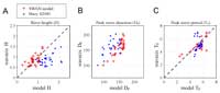 |
Figure 14. Model predictions of A, wave height (H), B, peak wave direction (Dp), and C, peak wave period (Tp) in the northern Gulf of Mexico alongshore Alabama and Florida for January 1525, 2007, compared with observations (wavecis) from a Naval Research Laboratory acoustic doppler current profiler at Santa Rosa Island, Florida. To demonstrate the accuracy of the model, we show the values from NDBC buoy 42040 offshore in the northern Gulf of Mexico as an alternative model for predicting nearshore values. Only cases where the measured nearshore wave height exceeded 0.5 meter are shown. |
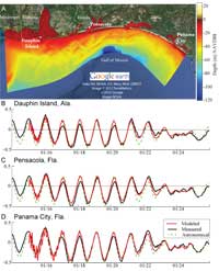 |
Figure 15. Evaluation of accuracy of simulated (modeled) water levels (in meters) against NOAA tidal measurements at A, three coastal inlet tide stations at B, Dauphin Island, Ala., C, Pensacola Pass, Fla., and D, Panama City Inlet, Fla. Astronomical water level predictions are also shown. The model predictions include some noise in the initial spinup of the flow simulations, which disappears after a few tidal cycles. |
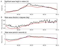 |
Figure 16. Simulated and measured wave characteristics at buoy 42012 (fig. 11) in the northern Gulf of Mexico alongshore Alabama and Florida during Hurricane Isaac in August 2012. Characteristics include A, significant wave height, B, mean wave direction, and C, mean wave period. |
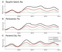 |
Figure 17. Simulation of water levels (in meters) in the northern Gulf of Mexico alongshore Alabama and Florida during Hurricane Isaac in August 2012 compared with measured water level at the NOAA tide stations at A, Dauphin Island, Ala., B, Pensacola, Fla., and C, Panama City, Fla. tide stations (fig. 15A) and to astronomical tide predictions. |
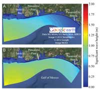 |
Figure 18. Significant wave height (table 2, metric 1) for scenarios A, H3_D6 and B, H3_D8 (fig. 2) in the northern Gulf of Mexico alongshore Alabama and Florida. Nearshore wave height in each scenario originated with 1- to 1.5-meter (m)-high waves at National Oceanic and Atmospheric Administration buoy 42040, but with southeasterly and south-southeasterly wind directions, respectively. |
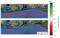 |
Figure 19. Maximum alongshore velocity (table 2, metric 2) smoothed over a 2-kilometer length scale for scenarios A, H3_D6 and B, H3_D8 (fig. 2) in the northern Gulf of Mexico alongshore Alabama and Florida. Green and red arrows indicate eastward- and westward-directed flows, respectively. Flow is to the west throughout the domain in A, whereas there are mixed flow directions in B. |
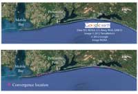 |
Figure 20. Flow convergence (table 2, metric 3) for scenarios A, H3_D6 and B, H3_D8 (fig. 2) in the northern Gulf of Mexico alongshore Alabama and Florida. Flow reversals are absent in A, whereas several flow reversals were identified in B and correspond to color changes in fig. 19B. |
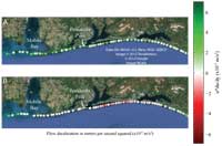 |
Figure 21. Flow deceleration (table 2, metric 4; as change, delta, d, meters per second squared, m/s2) for scenarios A, H3_D6 and B, H3_D8 (fig. 2) in the northern Gulf of Mexico alongshore Alabama and Florida. Spatial decelerations of varying magnitudes are found in both scenarios. |
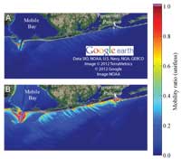 |
Figure 22. Mobility ratio (table 2, metric 5) in the northern Gulf of Mexico alongshore Alabama and Florida for a midlevel threshold of 2.5-centimeter surface residual balls (SRBs; table 1) for scenarios A, H3_D6 and B, H4_D6 (fig. 2). Areas with a mobility ratio of 1 (in pink) indicate where the mobility threshold was exceeded. Whereas the mobility threshold is exceeded only in small sections in very shallow water in A, the large wave heights result in mobility along the coast as well as over shallow bar and ebb tidal delta features in B . |
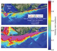 |
Figure 23. Mobility ratio (table 2, metric 5) in the northern Gulf of Mexico alongshore Alabama and Florida for sand for scenarios A, H3_D6 and B, H4_D6 (fig. 2). Areas with a mobility ratio of 1 (in pink) indicate where the mobility threshold was exceeded. Compared with 2.5-centimeter surface residual balls (SRBs; fig. 22), sand is mobile over a large portion of the domain in both scenarios, yielding the potential for exhumation and burial of SRBs in regions where the SRBs themselves are immobile. |
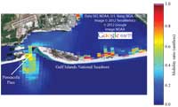 |
Figure 24. Mobility ratio (table 2, metric 5) in the northern Gulf of Mexico alongshore Alabama and Florida for a midlevel threshold of 2.5-centimeter (cm) surface residual balls (SRBs; table 1) along the Gulf Islands National Seashore (east of Pensacola Pass, Florida) for wave scenario H5_D1, corresponding to waves observed at NDBC buoy 42040 of height greater than 2 meters and coming from a north-northeasterly direction (fig. 2). Where the mobility ratio exceeded 1 (in pink) mobility of 2.5-cm SRBs was indicated at locations along the back-barrier from northerly wind-waves locally generated behind the barrier. |
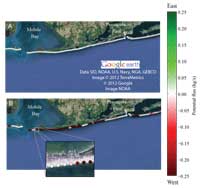 |
Figure 25. Surf-zone integrated alongshore potential flux smoothed over 2 kilometers (table 2, metric 6) for 2.5-centimeter surface residual balls (SRBs; table 1) in the northern Gulf of Mexico alongshore Alabama and Florida for scenarios A, H3_D6 and B, H4_D6. Because of the limited mobility in A (fig. 23), there is virtually no potential flux, whereas there is westward potential flux throughout the domain in B. Areas where the magnitude of the flow decreases (B, inset) are more likely areas of SRB deposition. |
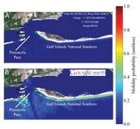 |
Figure 26. Weighted mobility probability (table 2, metric 7) from April 2010 to August 2012 along the Gulf Islands National Seashore (east of Pensacola Pass, Fla.) for 2.5-centimeter surface residual balls (SRBs). Shown is an estimate using A, the highest estimate of critical stress, appropriate for SRBs flush with the seabed, and B, the lowest estimate of critical stress, appropriate for SRBs sitting atop the seabed. |
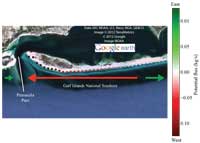 |
Figure 27. Weighted surf-zone integrated alongshore potential flux (table 2, metric 8), indicating the average potential flux in the northern Gulf of Mexico alongshore Alabama and Florida from April 2010 to August 2012 for 2.5-centimeter surface residual balls (SRBs; table 1) using a midrange estimate of critical stress. There is a convergence in the probable flux at Pensacola Pass, Fla., and divergence toward the east of Pensacola Pass. |
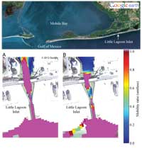 |
Figure 28. Tidal inlet surface residual ball (SRB) mobility (table 2, metric 9) at A, maximum flood and B, maximum ebb for 2.5-centimeter SRBs (table 1) using a low critical threshold at Little Lagoon Inlet, Ala. (fig. 1). Areas where the mobility ratio is 1 (in pink) indicate that the critical threshold for SRB mobility is exceeded. The greater extent of tidal inlet SRB mobility during flood increases the probability that SRBs brought in by the tide will remain trapped. Local surficial sediment is mobilized throughout the illustrated domain during both flood and ebb tide, leading to potential for burial and exposure of SRBs. |
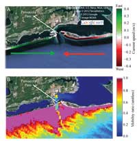 |
Figure 29. A, Maximum alongshore flow speed (green and red arrows) smoothed over a 2-kilometer length scale (table 2, metric 2) and B, mobility ratio (table 2, metric 5) using the lowest critical stress threshold, appropriate for surface residual balls (SRBs) sitting on top of the seabed, for 10-centimeter SRBs (table 1) near Pensacola Pass, Fla., for scenario H5_D8 (fig. 2). All small-size classes of SRBs are also mobilized, leading to convergence and a high probability of deposition in Pensacola Pass during the wave conditions represented by this scenario. |
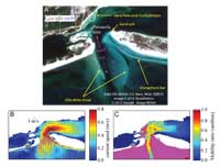 |
Figure 30. A, Morphologic features (yellow arrows) at the Pensacola Inlet, Fla., that interact with the tidal flow (pink arrowssolid arrows indicate flood tide flows and dashed arrows indicate ebb tide flows). B, Modeled inlet flow speeds and C, 2.5-centimeter surface residual ball (SRB) mobility for low threshold calculations during flood tide with moderately large waves (scenario H4_D7; fig. 2). Areas where the mobility ratio is 1 (in pink) indicate that SRB mobility threshold is exceeded. |
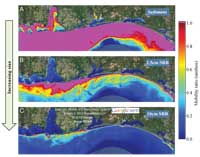 |
Figure 31. Mobility ratios (table 2, metric 5) of A, 0.03-centimeter (cm) quartz sand (sediment); and B, 2.5-cm and C, 10-cm surface residual balls (SRBs) under large wave (more than 2-meter) conditions in the northern Gulf of Mexico alongshore Alabama and Florida corresponding to scenario H5_D8 (fig. 2). Where the mobility ratio is 1 (pink areas), the SRB mobility threshold is exceeded. Sediment is more mobile than centimeter-sized SRBs, with mobility decreasing with increasing SRB size. |
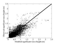 |
Figure 32. Observed wave height at the Naval Research Labortory acoustic dopler current profiler (ADCP) in the northern Gulf of Mexico alongshore Alabama and Florida for September 15, 2006, through December 23, 2007, against the reconstructed wave height using corresponding subset of modeled scenarios. |
|


