
|
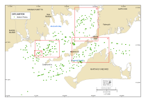 |
Figure 6. Map showing locations of bottom photographs, which were classified according to the Coastal and Marine Ecological Classification Standard (CMECS), specifically the Benthic Biotic Component. Red rectangles indicate areas of detail shown in figures 7, 9, 11, and 16. Is., Island; UTM, Universal Transverse Mercator; WGS 84, World Geodetic System of 1984. Click on figure for larger image. |
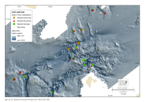 |
Figure 7. Map showing a high-relief area colonized by anemones, bryozoans, and sponges. See figure 6 for map location. See figure 8 for an example photograph (d3_PICT0864.JPG). Bathymetry is from U.S. Geological Survey Open-File Report 2012–1002. Is., Island; UTM, Universal Transverse Mercator; WGS 84, World Geodetic System of 1984. Click on figure for larger image. |
Biological Classification of the Photographs
Nearly all of the 2,426 sea-floor photographs taken during U.S. Geological Survey (USGS) Field Activity 2010–005–FA were reviewed and classified by Massachusetts Office of Coastal Zone Management (CZM) biologists according to the Coastal and Marine Ecological Classification Standard (CMECS), specifically the Benthic Biotic Component (Federal Geographic Data Committee, 2012). Of these, 2,265 photographs (fig. 6) were of suitable resolution for the benthic biology in their imagery to be classified.
CMECS is a hierarchal system that provides a way to classify ecological units by using a standard format. In the CMECS Benthic Biotic Component, biotic classification units are defined by the dominance of sessile or relatively nonmobile fauna; taxa with the greatest percent cover in the observational footprint are deemed the most dominant and are classified as the Biotic Group. Because additional taxa and groups of interest can co-occur with the dominant taxa group in any given photograph, two co-occurring biotic groups (Co-occurring Element Modifiers) and two associated taxa (Associated Taxa Modifiers) were added as modifiers to the classification scheme. Adding modifiers to the dominant biotic group increases the amount of biological information available from the imagery without adding a significant time burden to the visual analysis of the photographs.
The analyzed images are useful for creating maps of existing biological resources and identifying important habitat areas and habitat associations. For example, the classified images can be used to map and identify the following: areas of high relief and structure necessary for sessile organisms such as sponges and bryozoans to attach (figs. 7 and 8), areas of hard substrate at depths shallow enough to accommodate photosynthesis in benthic macroalgae (figs. 9 and 10), areas of soft sediment suitable for species such as those that burrow (figs. 9 and 10), and the distribution of nonnative species, can affect habitat quality (figs. 11, 12, and 13). The biological information derived from the digital photographs allows for a more complete assessment of benthic habitat conditions.
The biological information from the photographs might also improve the accuracy of bottom-type interpretation. For example, heavy accumulations of Crepidula sp. could be incorrectly interpreted as hard bottom, on the basis of the backscatter intensity data alone (figs. 14 and 15). Relief created from benthic species such as soft-sediment sponges and hard corals that would not necessarily be identified as structure in a geological context can also be mapped (figs. 16, 17, 18, and 19).
The classification of the benthic biota is included in the bottom-photographs dataset. These data are available as a spreadsheet, shapefile, or Google Earth KMZ file (fig. 20) in appendix 1 (Geospatial Data). Additional information about the classification process and its accuracy can be found in the metadata for the bottom-photographs dataset in appendix 1 (Geospatial Data).
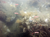
Figure 8. Photograph d3_PICT0864.JPG, taken along SEABed Observation and Sampling System (SEABOSS) video trackline 112, of bryozoans, anemones, sponges, Astrangia sp. (hard coral), and other species colonizing hard substrate. See figure 7 for photograph location. Scale of the photographs are generally 0.5 to 1.0 meters across, depending on the height of the SEABOSS when the photograph was taken. The scale of this photograph is 80 centimenters across. Click on figure for larger image.
|
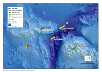
Figure 9. Map showing a channel feature and the distribution of primarily soft-sediment species within the channel and benthic macroalgae (seaweeds) and other attached sessile species in the areas of higher elevation and relief. See figure 6 for map location. See figure 10 for example photographs (A, d3_PICT1168.JPG; B, d3_PICT1183.JPG; C, d3_PICT1176.JPG; D, d3_PICT1160.JPG). Bathymetry is from U.S. Geological Survey Open-File Report 2012–1002. UTM, Universal Transverse Mercator; WGS 84, World Geodetic System of 1984. Click on figure for larger image.
|
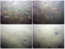
Figure 10. Photographs of A, attached fauna west of the channel, B, benthic macroalgae east of the channel, C, soft-sediment fauna in the channel, and D, soft-sediment fauna at the mouth of the channel. See figure 9 for photograph locations. Photograph A, d3_PICT1168.JPG, taken along SEABed Observation and Sampling System (SEABOSS) video trackline 156; B, d3_PICT1183.JPG, trackline 158; C, d3_PICT1176.JPG, trackline 157; D, d3_PICT1160.JPG, trackline 155. The scale of these photographs are A, 80 centimeters (cm) across; B, 60 cm; C 50 cm; D, 60 cm.Click on figure for larger image.
|
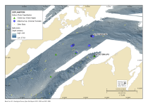
Figure 11. Map showing the distribution of nonnative species, including Codium fragile (likely Codium fragile ssp. fragile)and Didemnum sp. (likely Didemnum vexillum), identified in the classified bottom photographs. See figure 6 for map location. See figures 12 and 13 for example photographs (d4_PICT2252.JPG and d4_PICT2569.JPG, respectively). Bathymetry is from U.S. Geological Survey Open-File Reports 2012–1002 and 2012–1006. UTM, Universal Transverse Mercator; WGS 84, World Geodetic System of 1984. Click on figure for larger image. |
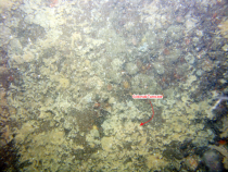
Figure 12. Photograph d4_PICT2252.JPG, taken along SEABed Observation and Sampling System (SEABOSS) video trackline 272, of a colonial tunicate, likely nonnative Didemnum vexillum, on cobbles in Vineyard Sound. See figure 11 for photograph location. The scale of this photograph is 1 meter across. Click on figure for larger image. |
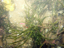
Figure 13. Photograph d4_PICT2569.JPG, taken along SEABed Observation and Sampling System (SEABOSS) video trackline 300, of the green algae Codium sp., likely the nonnative Codium fragile ssp. fragile. See figure 11 for photograph location. The scale of this photograph is 80 centimeters across. Click on figure for larger image. |
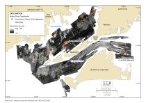
Figure 14. Map showing Crepidula sp. (slipper shell) aggregations overlaid on backscatter intensity. See figure 15 for example photographs (A, d3_PICT0683.JPG; B, d4_PICT2415.JPG; C, d4_PICT2420.JPG). Backscatter imagery is from U.S. Geological Survey Open-File Reports 2012–1002 and 2012–1006. Is., Island; UTM, Universal Transverse Mercator; WGS 84, World Geodetic System of 1984. Click on figure for larger image. |
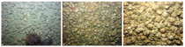
Figure 15. Photographs of Crepidula sp. (slipper shell) aggregations, including reef formations (B and C). See figure 14 for photograph locations. A, Photograph d3_PICT0683.JPG, taken along SEABed Observation and Sampling System (SEABOSS) video trackline 94; B, d4_PICT2415.JPG, trackline 282, C: d4_PICT2420.JPG, trackline 282. The scale of these photographs are A, 60 centimeters (cm) across; B, 65 cm; C, 40 cm. Click on figure for larger image. |
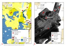
Figure 16. Maps showing soft-sediment sponges overlaid on A, sediment phi class, and B, backscatter intensity. See figure 6 for map location. See figure 17 for an example photograph (d1_PICT0447.JPG). Sediment phi classes are from U.S. Geological Survey Open-File Report 2014–1220 (Foster and others, 2014). Backscatter imagery from USGS Open-File Report 2012–1002. UTM, Universal Transverse Mercator; WGS 84, World Geodetic System of 1984. Click on figure for larger image. |
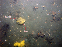
Figure 17. Photograph d1_PICT0447.JPG, taken along SEABed Observation and Sampling System (SEABOSS) video trackline 018, of Cliona sp. (sponge) and Crepidula sp. (slipper shell) on primarily soft substrate. See figure 16 for photograph location. The scale of this photograph is 60 centimeters across. Click on figure for larger image. |
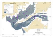
Figure 18. Map showing Astrangia sp. (hard coral) distribution. See figure 19 for an example photograph (d4_PICT1679.JPG). Bathymetry is from USGS Open-File Reports 2012–1002 and 2012–1006. Is., Island; UTM, Universal Transverse Mercator; WGS 84, World Geodetic System of 1984. Click on figure for larger image. |
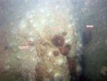
Figure 19. Photograph d4_PICT1679.JPG, taken along SEABed Observation and Sampling System (SEABOSS) video trackline 217b, of Astrangia sp. (hard coral) on a boulder. Arbacia punctulata (purple sea urchin) and Homarus americanus (American lobster) are also pictured. See figure 18 for photograph location.The scale of this photograph is approximately 60 centimeters across. Click on figure for larger image. |
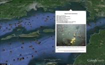
Figure 20. Screen capture of the Google Earth KMZ file that contains the Coastal and Marine Ecological Classification Standard (CMECS) classification of the bottom photographs. Click on figure for larger image. |
|

