| List of Figures
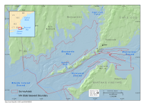 |
Figure 1. Map showing the location of the area targeted for sampling (outlined in red) offshore of Massachusetts in Buzzards Bay and Vineyard Sound. Sampling was generally done in the area coincident with newly acquired geophysical data from 2009 and 2010. MOF, [U.S. Geological Survey] Marine Operations Facility; UTM, Universal Transverse Mercator; WGS 84, World Geodetic System of 1984. |
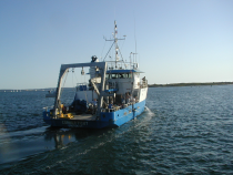 |
Figure 2. Photograph of the research vessel (RV) used for the sampling survey, the RV Connecticut. |
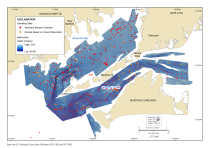 |
Figure 3. Map showing SEABed Observation and Sampling System (SEABOSS) sampling sites (red dots) over depth-colored shaded-relief topography of the sea floor in the study area. Bathymetry is from U.S. Geological Survey Open-File Reports 2012–1002 and 2012–1006. Is., Island; UTM, Universal Transverse Mercator; WGS 84, World Geodetic System of 1984. |
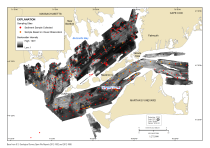 |
Figure 4. Map showing SEABed Observation and Sampling System (SEABOSS) sampling sites (red dots) overlaid on acoustic-backscatter intensity in the study area. Backscatter intensity is an acoustic measure of the relative hardness and roughness of the sea floor. In general, high values (light tones) represent rock, boulders, cobbles, gravel, and coarse sand. Low values (dark tones) generally represent fine sand and muddy sediment. Tonal variations can occur across track in the sidescan-sonar data as a result of changes in acquisition or processing parameters. Backscatter imagery is from U.S. Geological Survey Open-File Reports 2012–1002 and 2012–1006. Is., Island; UTM, Universal Transverse Mercator; WGS 84, World Geodetic System of 1984. |
|
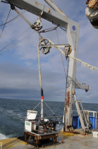
Figure 5. Photograph of the SEABed Observation and Sampling System (SEABOSS) during survey 2010–005 aboard the research vessel Connecticut. The SEABOSS system was used to collect video, photographic data, and sediment samples. |
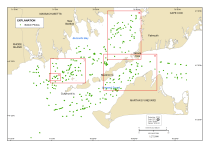 |
Figure 6. Map showing locations of 2,426 bottom photographs, which were classified according to the Coastal and Marine Ecological Classification Standard (CMECS), specifically the Benthic Biotic Component. Red rectangles indicate areas of detail shown in figures 7, 9, 11, and 16. Is., Island; UTM, Universal Transverse Mercator; WGS 84, World Geodetic System of 1984. |
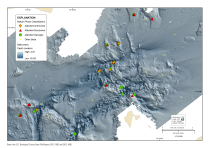 |
Figure 7. Map showing a high-relief area colonized by anemones, bryozoans, and sponges. See figure 6 for map location. See figure 8 for an example photograph (d3_PICT0864.JPG). Bathymetry is from U.S. Geological Survey Open-File Report 2012–1002. Is., Island; UTM, Universal Transverse Mercator; WGS 84, World Geodetic System of 1984. |
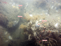 |
Figure 8. Photograph d3_PICT0864.JPG, taken along SEABed Observation and Sampling System (SEABOSS) video trackline 112, of bryozoans, anemones, sponges, Astrangia sp. (hard coral), and other species colonizing hard substrate. See figure 7 for photograph location. Scale of the photographs are generally 0.5 to 1.0 meters across, depending on the height of the SEABOSS when the photograph was taken. The scale of this photograph is 80 centimenters across. |
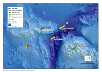 |
Figure 9. Map showing a channel feature and the distribution of primarily soft-sediment species within the channel and benthic macroalgae (seaweeds) and other attached sessile species in the areas of higher elevation and relief. See figure 6 for map location. See figure 10 for example photographs (A, d3_PICT1168.JPG; B, d3_PICT1183.JPG; C, d3_PICT1176.JPG; D, d3_PICT1160.JPG). Bathymetry is from U.S. Geological Survey Open-File Report 2012–1002. UTM, Universal Transverse Mercator; WGS 84, World Geodetic System of 1984. |
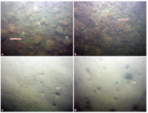 |
Figure 10. Photographs of A, attached fauna west of the channel, B, benthic macroalgae east of the channel, C, soft-sediment fauna in the channel, and D, soft-sediment fauna at the mouth of the channel. See figure 9 for photograph locations. Photograph A, d3_PICT1168.JPG, taken along SEABed Observation and Sampling System (SEABOSS) video trackline 156; B, d3_PICT1183.JPG, trackline 158; C, d3_PICT1176.JPG, trackline 157; D, d3_PICT1160.JPG, trackline 155. The scale of these photographs are A, 80 centimeters (cm) across; B, 60 cm; C 50 cm; D, 60 cm. |
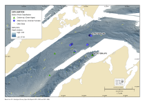 |
Figure 11. Map showing the distribution of nonnative species, including Codium fragile (likely Codium fragile ssp. fragile)and Didemnum sp. (likely Didemnum vexillum), identified in the classified bottom photographs. See figure 6 for map location. See figures 12 and 13 for example photographs (d4_PICT2252.JPG and d4_PICT2569.JPG, respectively). Bathymetry is from U.S. Geological Survey Open-File Reports 2012–1002 and 2012–1006. UTM, Universal Transverse Mercator; WGS 84, World Geodetic System of 1984. |
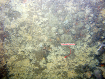 |
Figure 12. Photograph d4_PICT2252.JPG, taken along SEABed Observation and Sampling System (SEABOSS) video trackline 272, of a colonial tunicate, likely nonnative Didemnum vexillum, on cobbles in Vineyard Sound. See figure 11 for photograph location. The scale of this photograph is 1 meter across. |
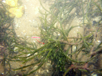 |
Figure 13. Photograph d4_PICT2569.JPG, taken along SEABed Observation and Sampling System (SEABOSS) video trackline 300, of the green algae Codium sp., likely the nonnative Codium fragile ssp. fragile. See figure 11 for photograph location. The scale of this photograph is 80 centimeters across. |
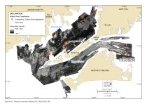 |
Figure 14. Map showing Crepidula sp. (slipper shell) aggregations overlaid on backscatter intensity. See figure 15 for example photographs (A, d3_PICT0683.JPG; B, d4_PICT2415.JPG; C, d4_PICT2420.JPG). Backscatter imagery is from U.S. Geological Survey Open-File Reports 2012–1002 and 2012–1006. Is., Island; UTM, Universal Transverse Mercator; WGS 84, World Geodetic System of 1984. |
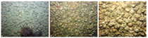 |
Figure 15. Photographs of Crepidula sp. (slipper shell) aggregations, including reef formations (B and C). See figure 14 for photograph locations. A, Photograph d3_PICT0683.JPG, taken along SEABed Observation and Sampling System (SEABOSS) video trackline 94; B, d4_PICT2415.JPG, trackline 282, C: d4_PICT2420.JPG, trackline 282. The scale of these photographs are A, 60 centimeters (cm) across; B, 65 cm; C, 40 cm. |
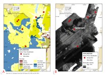 |
Figure 16. Maps showing soft-sediment sponges overlaid on A, sediment phi class, and B, backscatter intensity. See figure 6 for map location. See figure 17 for an example photograph (d1_PICT0447.JPG). Sediment phi classes are from U.S. Geological Survey Open-File Report 2014–1220 (Foster and others, 2014). Backscatter imagery from USGS Open-File Report 2012–1002. UTM, Universal Transverse Mercator; WGS 84, World Geodetic System of 1984. |
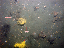 |
Figure 17. Photograph d1_PICT0447.JPG, taken along SEABed Observation and Sampling System (SEABOSS) video trackline 018, of Cliona sp. (sponge) and Crepidula sp. (slipper shell) on primarily soft substrate. See figure 16 for photograph location. The scale of this photograph is 60 centimeters across. |
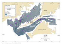 |
Figure 18. Map showing Astrangia sp. (hard coral) distribution. See figure 19 for an example photograph (d4_PICT1679.JPG). Bathymetry is from USGS Open-File Reports 2012–1002 and 2012–1006. Is., Island; UTM, Universal Transverse Mercator; WGS 84, World Geodetic System of 1984. |
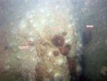 |
Figure 19. Photograph d4_PICT1679.JPG, taken along SEABed Observation and Sampling System (SEABOSS) video trackline 217b, of Astrangia sp. (hard coral) on a boulder. Arbacia punctulata (purple sea urchin) and Homarus americanus (American lobster) are also pictured. See figure 18 for photograph location. The scale of this photograph is approximately 60 centimeters across. |
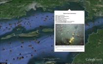 |
Figure 20. Screen capture of the Google Earth KMZ file that contains the Coastal and Marine Ecological Classification Standard (CMECS) classification of the bottom photographs. |
|