U.S. Geological Survey Open-File Report 2010-1091
High-Resolution Geophysical Data Collected Within Red Brook Harbor, Buzzards Bay, Massachusetts, in 2009
|
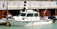
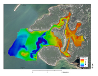
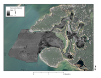
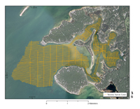
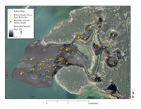
The Red Brook Harbor survey area was approximately 7 km2, with depths ranging from 0 to approximately 10 m. Surveying was conducted aboard the R/V Rafael (fig. 2), a 25-foot single-hull vessel equipped with an interferometric sonar system for mapping bathymetry and backscatter, a compressed high-intensity radar pulse (CHIRP) seismic reflection profiler to collect sub-bottom data, a sound velocity profiler to acquire speed of sound within the water column, and a sea floor sampling device to collect sediment samples, video, and photographs. Survey operations were conducted over the course of 13 days, from September 28 through November 17, 2009. HYPACK Survey (HYPACK, Inc., 2010) was used for survey line planning and vessel positioning during survey operations. Vessel positions were determined with a differential global positioning system (DGPS) and were recorded in HYPACK Survey. Acoustic data were collected along approximately 240 kilometers (km) of survey lines. Survey lines were spaced 30 m apart, with orthogonal and oblique tie lines acquired at approximately 300-m spacing (fig. 5).Swath BathymetryBathymetric data were collected with an SEA SWATHplus 234-kilohertz (kHz) interferometric sonar system (SEA, undated). Vessel motion (heave, pitch, roll, and yaw) was recorded with a CodaOctopus F180 attitude and positioning system (CodaOctopus Products Ltd., 2010). The SWATHplus transducers and the Octopus F180 were mounted on the bow of the R/V Rafael on a rigid, vertical pole, with the Octopus F180 mounted directly above the SWATHplus transducers. The speed of sound at the transducer face was monitored continuously with an AML Oceanographic Micro SV velocimeter (AML Oceanographic, 2010) mounted at the sonar heads. Two real-time kinematic (RTK) navigation antennas and a DGPS navigation antenna were mounted on a cross-bar atop the vertical pole mount, directly above the transducers and the Octopus F180. Horizontal and vertical offsets between the DGPS antennas and the Octopus F180 and the SWATHplus transducers were applied and recorded in the Octopus F180 and SWATHplus configuration files. DGPS navigation was used to record horizontal and vertical positions of the soundings during acquisition. RTK corrections were broadcast to the survey vessel once every second from a base station established by USGS personnel in the inner harbor, providing more precise positioning of the RTK anenna (with accuracy of 20 centimeters (cm) or better). Horizontal RTK positions will be merged with the SWATHplus bathymetric data for a future data release. RTK-measured vertical heights were used to correct tidal offsets during post-processing. Bathymetry tracklines can be downloaded from appendix 1 (Geospatial Data). Initial processing of bathymetric data was performed with SWATHplus acquisition and processing software. Vessel motion data recorded by the Octopus F180 were used to correct offsets resulting from heave, pitch, roll and yaw of the vessel, and filters were applied to remove spurious soundings. Sound velocity profiles (SVP) of the water column were acquired with an AML Oceanographic SV Plus V2 velocimeter (AML Oceanographic, 2010). Profiles were collected at least once during each survey day and multiple times per day when the data suggested significant stratification within the water column (fig. 6). Sound velocity profiles were applied within SWATHplus software during processing to correct bathymetric soundings for errors resulting from changes in the speed of sound within the water column. SVP locations and raster (JPEG) images for each profile are available for download in appendix 1 (Geospatial Data). Following processing in SWATHplus, soundings were imported into CARIS hydrographic information processing system software HIPS (CARIS, 2010) for further processing. RTK-corrected tide values were applied to reference soundings to mean lower low water (MLLW), and remaining spurious soundings were removed by further filtering and manual editing where needed. Continuous bathymetric surfaces were created at 1- and 5- m per pixel (mpp) grids and were exported from CARIS in ASCII format for import into Environment Systems Research Institute (ESRI) grid format (Environmental Systems Research Institute, 2010). Corresponding georeferenced color-shaded relief TIFF images of the bathymetry were created at 1- and 5-mpp resolution for use in data visualization and presentation. The ESRI grid data and the color-shaded relief images of the bathymetry can be downloaded from appendix 1 (Geospatial Data). Figure 7 shows a color-shaded relief image of the bathymetry for Red Brook Harbor. Acoustic BackscatterAcoustic backscatter, a measure of the intensity of returns from an insonified area of the sea floor, was recorded by the SEA SWATHplus interferometric sonar system. SXPTOOLS software (Finlayson, 2009) was used to enhance the visual quality of the SWATHplus interferometric backscatter data by applying an empirical gain normalization (EGN) function to optimize the dynamic range of recorded intensities. SXPTOOLS was also used to interpolate across data gaps at nadir that resulted from the filtering techniques applied to the bathymetric soundings. Chesapeake Technology, Inc. SonarWiz software (Chesapeake Technology, Inc., undated) was used to mosaic the backscatter data and export 1- and 5-mpp georeferenced TIFF images. Backscatter images are provided for download in appendix 1 (Geospatial Data). Figure 8 shows the backscatter imagery for Red Brook Harbor. Low backscatter values are shown in dark tones and generally represent finer sediment or relatively soft sea floor. High backscatter returns are shown in lighter tones and generally represent relatively coarser sediment or hard sea floor.Seismic ReflectionSeismic reflection profiles were collected with a Knudsen Engineering, Ltd. (KEL) Chirp 3202 dual-frequency (centered at 3.5- and 200-kHz) CHIRP system (Knudsen Engineering, Ltd., undated) with transducers mounted on a rigid pole on the starboard side of the survey vessel. The transducer draft was 0.5 m below the water surface, and the draft offset was accounted for during data acquisition. Single-beam water depths from the 200-kHz channel were logged together with DGPS navigation in ASCII format. Seismic-reflection data with peak frequencies of 3.5 or 5 kHz were recorded to Society of Exploration Geophysicists Y (SEG-Y) format (Barry and others, 1975) with DGPS navigation logged to the SEG-Y file trace headers. The Chirp 3202 was fired at a rate of 0.2 or 0.25 seconds and set to record trace lengths between 26 and 130 milliseconds. A total of 240 linear km of seismic data was collected. The SIOSEIS software (University of California, San Diego, undated) was used to mute the water column portions of the seismic traces using the water depths recorded in the 200-kHz channel and to apply gain and automatic gain control functions to traces. Seismic Unix (Colorado School of Mines, 2010) was used to read navigation data from trace headers and plot the data as JPEG images (fig. 9). Figure 10 shows seismic tracklines for the Red Brook Harbor survey. Seismic tracklines, shot points, and profile images can be downloaded from appendix 1 (Geospatial Data). Bottom Samples and PhotographyThe USGS Mini SEABed Observation and Sampling System (Mini SEABOSS; Valentine and others, 2000; Blackwood and Parloski, 2001) was used to collect digital photography and video and sediment samples at 48 sites within the study area. Mini SEABOSS data are used to investigate how spatial variability in sea floor character and composition relate to acoustic variability in the geophysical data. Areas of transition between high and low backscatter and large areas of homogeneous backscatter were chosen for 24 of the sample sites. The remaining 24 sample sites were selected randomly using a geographic information system (GIS) routine and will be used in future habitat modeling efforts. Photographs, video, and sediment samples were collected as the vessel drifted at a speed of less than 1 knot (nautical mile) over the sample sites. Approximately 5 to 10 photographs were acquired for each site; the sediment sample was collected at the end of each drift. Thick shell cover prevented sample grabs at seven stations in the outer harbor. The upper 2 cm of sediment was bagged and later analyzed for grain size and other physical characteristics in a USGS sediment analysis laboratory (Poppe and others, 2005). Sea floor composition prohibited acquiring bottom samples at seven of the planned sites in the outer harbor. Figure 11 shows the location of sediment samples and digital photographs. Bottom sample locations with sediment analysis results and photograph locations are included for download in shapefile format in appendix 1 (Geospatial Data).
|
|