U.S. Geological Survey Open-File Report 2015-1153
MethodsOverviewThis section describes how the interpretations presented in this report were generated. Detailed descriptions of software, source information, scale, and accuracy assessments for each dataset are provided in the metadata files for geospatial data layers in appendix 1. Geophysical DataThe data sources for swath bathymetry, lidar, and backscatter are the same as those presented in Pendleton and others (2013) (figs. 3 and 4; table 2). Rugosity derived by using DEM Surface Tools (Jenness Enterprises, 2015) and bathymetric gradient were calculated at the highest resolution of each survey (table 2). Shaded relief images were created from bathymetry exaggerated two times and illuminated with a light source from 315 degrees (°) at an elevation of 45°. Table 2. Data sources for the digital elevation model, backscatter mosaic, and seismic-reflection profile interpretations.
*These data were not used in the composite backscatter image. Previous InterpretationsPhysiographic zone and seismic cross-sectional interpretations for nearshore areas between Nahant and Gloucester and Cape Ann and Salisbury are presented in Barnhardt and others (2006, 2009). Oldale and Bick (1987), Oldale and Wommack (1987), and Oldale and others (1994) presented geologic interpretations for parts of Massachusetts Bay and the inner continental shelf offshore of Cape Ann to New Hampshire. Butman and others (2006a-c; 2007) produced sea-floor topography maps and feature descriptions in western Massachusetts Bay. Hein and others (2013) produced an onshore/offshore geologic map of Newburyport and Ipswich, Mass., extending to about 90 m water depth. Seismic units from previously published geologic and stratigraphic interpretations were combined, providing an input map layer (surficial geologic and stratigraphic interpretations) for this study (fig. 5). Not all of the previously published geologic and stratigraphic maps were created at the same resolution, nor did they use the same naming convention for the stratigraphic units mapped. Figure 6 summarizes how the units used in previous studies were combined in this study into generalized geologic units in order to produce a map layer to inform sediment texture and physiographic zone interpretations. Sediment Samples and Sediment Texture Classification SchemesSediment sample databases of Ford and Voss (2010) and McMullen and others (2011) were supplemented with National Oceanic and Atmospheric Administration chart sampling data and more than 1,700 bottom photographs and descriptions (fig. 7; Gutierrez and others, 2000; Barnhardt and others 2006, 2009; Emily Huntley, CZM, unpub. data, 2012). This study uses the Barnhardt and others (1998) sediment texture classification scheme (fig. 8). The Barnhardt and others (1998) system is based on four basic, easily recognized sediment units (as measured in grain size, based on Wentworth, 1922): rock (R; grain size greater than 64 millimeters [mm]), gravel (G; grain size greater than 2 to 64 mm), sand (S; grain size of 0.062 mm to 2 mm), and mud (M; grain size less than 0.062 mm). Because the sea floor is often not a uniform mixture of these units, the classification is further divided into 12 composite units, which are two-part combinations of the 4 basic units (fig. 8). This classification is defined such that the primary texture, representing more than 50 percent of an area's texture, is given an uppercase letter, and the secondary texture, representing less than 50 percent of an area's texture, is given a lowercase letter. If one of the basic sediment units represents more than 90 percent of the texture, only its uppercase letter is used. The units defined under the Barnhardt and others (1998) classification within this study area include R, gravelly rock (Rg), sandy rock (Rs), and muddy rock (Rm); G, rocky gravel (Gr), sandy gravel (Gs), and muddy gravel (Gm); S, gravelly sand (Sg), muddy sand (Sm), and rocky sand (Sr); and M, rocky mud (Mr), gravelly mud (Mg), and sandy mud (Ms). Sediment Texture MappingThe texture and spatial distribution of sea-floor sediment were mapped qualitatively in ArcGIS by using acoustic-backscatter intensity, bathymetry, lidar, geologic interpretations, aerial photography, bottom photographs, and sediment samples. The mapping was done by using the highest data resolution available, typically 2 m in water depths less than 30 m, and 10 m for water depths greater than 30 m. First, sediment texture polygons were outlined by using backscatter intensity data to define changes in the sea floor based on acoustic return (figs. 3 and 9A). Areas of high backscatter intensity (light tones) have strong acoustic reflections, suggest boulders and gravels, and generally are characterized by coarse sea-floor sediments. Low-backscatter-intensity areas (dark tones) have weak acoustic reflections and generally are characterized by fine-grained material such as muds and fine sands. The polygons were then refined and edited by using gradient, rugosity, and hillshaded relief images derived from interferometric and multibeam swath bathymetry and from lidar at the highest resolution available (figs. 4 and 9B–E). Areas of rough topography and high rugosity typically are associated with rocky areas, whereas smooth, low-rugosity regions tend to be blanketed by fine-grained sediment. These bathymetric derivatives helped to refine polygon boundaries where changes from areas of primarily rock to areas of primarily gravel may not have been apparent in backscatter data but could easily be identified in hillshaded relief, rugosity and slope data (figs. 9 and 10). Finally, bottom photographs and sediment samples (fig. 7) were used to define sediment texture for each polygon that was drawn by using geophysical data (fig. 10). Percentages of gravel, sand, silt, and clay and phi size for each sediment texture polygon were calculated by using grain-size statistics of laboratory-analyzed sediment samples within the defined polygon. Texture data based on laboratory grain-size analysis were preferred over visual descriptions when defining sediment texture throughout the study area. Of the more than 6,000 samples in total within the study area, 1,215 were analyzed in the laboratory for grain size (fig. 7). Sediment texture statistics for each polygon can be found within the geospatial data file (Nahant_NH_sedcover.shp) for sediment texture in appendix 1. The number of sediment samples in a polygon ranged from 0 to 166. For multiple samples within a polygon, the dominant sediment texture (as defined by Barnhardt and others [1998]) or average phi size, when available) was used to classify sediment type. Average phi size and average particle content by weight data were not typically representative and frequently not available in rock and gravel areas because the grab sampler could not sample the range of sediment sizes on the sea floor because of large particles. In these areas, bottom photographs were used in the absence of sediment samples to qualitatively define sediment texture. The average texture statistics are most representative in polygons with several samples and textures in the sand and smaller sediment classes. Polygons that lacked sample information (23 percent of the interpreted area) were defined texturally through extrapolation from adjacent or proximal polygons of similar acoustic character that did contain sediment samples (77 percent of interpreted area). Physiographic ZonesThe sea floor within the study area was divided into physiographic zones by following the methods used in other parts of the Gulf of Maine (Kelley and Belknap, 1991; Kelley and others, 1996; Barnhardt and others, 2006, 2009; and Pendleton and others, 2013). The distribution of sea-floor physiographic zones was analyzed qualitatively in ArcGIS by using the same input sources and digitization techniques used to determine sediment texture and distribution (figs. 9 and 10). Physiographic zones identified within the study area include rocky zones, outer basins, nearshore basins, ebb-tidal deltas, hard-bottom plains, nearshore ramps, and shelf valleys. |
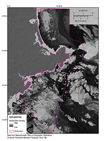 Figure 3. A composite backscatter image of the study area at 10-meter resolution, created from a series of published backscatter images (table 2). Areas of high backscatter intensity (light tones) have strong acoustic reflections and suggest boulders, gravels, and generally coarse sea-floor sediments. Areas of low backscatter intensity (dark tones) have weak acoustic reflections and are generally of finer grained material such as muds and fine sands. Regularly spaced striping is an artifact of the surveys. 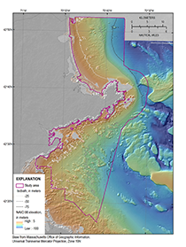 Figure 4. A digital elevation model (DEM), produced from swath-interferometric and multibeam bathymetry and lidar at 30-meter resolution (table 2). High rugosity and relief are most often associated with rocky areas, whereas smooth, low-relief regions tend to be blanketed by fine-grained sediment deposits. NAVD 88, North American Vertical Datum of 1988. 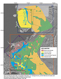 Figure 5. Generalized geologic map created by combining previously published stratigraphic interpretations within the study area and new interpretation for western Massachusetts Bay. Data are modified from (A) Barnhardt and others, 2006; (B) Oldale and Bick, 1987; (C) Oldale and Wommack, 1987; (D) Hein and others, 2013; and (E) Oldale and others, 1994. The stratigraphic correlation of units in this map is shown in figure 6. The drumlins identified by Oldale and others (1994) in western Massachusetts Bay are outlined in gray. 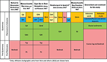 Figure 6. Seismic stratigraphic units interpreted by Oldale and Bick (1987), Oldale and Wommack (1987), and Hein and others (2013). Barnhardt and others (2006) published a depth to sediment thickness map, which was used to identify areas of outcropping bedrock on the inner continental shelf between Nahant and Gloucester, Massachusetts. Transgressive (thick red line) and regressive unconformities (dashed red line) were also identified in several of these studies. The stratigraphic unit names and resolution of these studies differed, but the origin and texture of the deposits can be readily combined into a generalized geologic map (fig. 5) to correlate with sediment textures and physiographic zones presented in this study. QbB and QhbC, Holocene beach and bar deposits; QssD, late Pleistocene to Holocene transgressive sand sheet deposits; QsrtD, late Pleistocene to Holocene regressive-transgressive shoreline deposits; QedD, Holocene ebb tidal delta deposits, QocD, late Pleistocene to Holocene offshore coarse deposits; QmB, QhmC, QmmE, and QmscD, late Pleistocene to Holocene offshore marine deposits; QfeB and QhfC, Holocene fluvial and estuarine deposits; QhdC, Holocene deltaic deposits; QdlD, late Pleistocene lowstand delta deposits; QdB and QmdC, Pleistocene glacial-marine deposits; QdoB and QdtC, Pleistocene coarse drift deposits; QtdD and QtE, Pleistocene drumlin till deposits; TcpB,C, Tertiary and late Cretaceous coastal plain deposits; Pz B,C, Triassic and older bedrock. 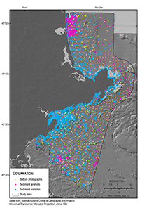 Figure 7. Bottom photographs (Barnhardt and others, 2006, 2009; Gutierrez and others, 2000; green dots) and sediment samples collected within the study area and used to aid interpretations. Sediment samples with laboratory analysis are shown as magenta dots, while blue dots are visual descriptions (Ford and Voss, 2010; McMullen and others, 2011; Emily Huntley, Massachusetts Office of Coastal Zone Management, unpub. data, 2012). 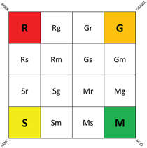 Figure 8. Barnhardt and others (1998) bottom-type classification based on four basic sediment units: Rock (R), Gravel (G), Sand (S), and Mud (M). If one of the basic sediment units represents more than 90 percent of the texture, only its uppercase letter is used. Twelve additional two-part units represent combinations of the four basic units, where the primary texture (greater than 50 percent) is given an uppercase letter and the secondary texture (less than 50 percent) is given a lowercase letter.  Figure 9. Sediment texture polygons were created in ArcGIS by using A, backscatter data, where areas of high backscatter intensity (light tones) have strong acoustic reflections and suggest boulders, gravels, and generally coarse sea-floor sediments ,and areas of low backscatter intensity (dark tones) have weak acoustic reflections and generally are characterized by fine-grained material such as muds and fine sands; B, hillshaded relief imagery, which creates a three-dimensional effect to provide a sense of topographic relief; C, rugosity, where blue polygons outline areas of variation or frequent amplitude changes in topography, often referred to as surface roughness; D, slope, where warm colors represent steeper areas of the map and cool colors represent flatter areas; and E, pseudocolored multibeam backscatter intensity(Butman and others, 2007), which combines backscatter and hillshaded relief. Each data type can provide useful information in a given area when defining texture boundaries. F, Bottom samples and photographs are used to assign a sediment texture within each polygon drawn on the basis of geophysical data and derivatives such as B–E. 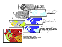 Figure 10. Sediment texture and distribution data were mapped qualitatively in ArcGIS by using a hierarchical methodology. Backscatter data were the first input, followed by bathymetry, surficial geologic and shallow stratigraphic interpretations, and photograph and sample databases. DEM, digital elevation model. From Pendleton and others (2013). |

![]() U.S. Department of the Interior |
U.S. Geological Survey
U.S. Department of the Interior |
U.S. Geological Survey
URL: http://pubsdata.usgs.gov/pubs/of/2015/1153/html/ofr20151153_methods.html
Page Contact Information: GS Pubs Web Contact
Page Last Modified: Wednesday, 07-Dec-2016 21:45:31 EST
