
| List of Figures
 |
Figure 1. Image of the study area (outlined in pink) that extends from offshore of Hull to Salisbury, Massachusetts, near the New Hampshire border. The outline is the extent of the surficial-sediment texture map and includes western Massachusetts Bay and the southern Merrimack Embayment. |
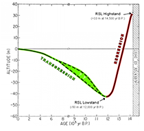 |
Figure 2. Sea-level curve for the southern Merrimack Embayment from Barnhardt and others (2009), modified after Oldale and others (1993). Following deglaciation, relative sea-level (RSL) fell in northeast Massachusetts in response to ice removal. Near the end of the Pleistocene, about 12,000 years before present (yr B.P.), sea level reached a lowstand of about -50 meters (m) before it began to rise again. Note the age scale changes at 8,000 yr B.P. |
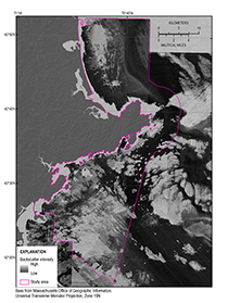 |
Figure 3. A composite backscatter image of the study area at 10-meter resolution, created from a series of published backscatter images (table 2). Areas of high backscatter intensity (light tones) have strong acoustic reflections and suggest boulders, gravels, and generally coarse sea-floor sediments. Areas of low backscatter intensity (dark tones) have weak acoustic reflections and are generally of finer grained material such as muds and fine sands. Regularly spaced striping is an artifact of the surveys. |
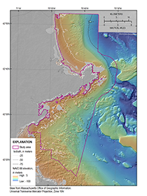 |
Figure 4. A digital elevation model (DEM), produced from swath-interferometric and multibeam bathymetry and lidar at 30-meter resolution (table 2). High rugosity and relief are most often associated with rocky areas, whereas smooth, low-relief regions tend to be blanketed by fine-grained sediment deposits. NAVD 88, North American Vertical Datum of 1988. |
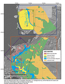 |
Figure 5. Generalized geologic map created by combining previously published stratigraphic interpretations within the study area and new interpretation for western Massachusetts Bay. Data are modified from (A) Barnhardt and others, 2006; (B) Oldale and Bick, 1987; (C) Oldale and Wommack, 1987; (D) Hein and others, 2013; and (E) Oldale and others, 1994. The stratigraphic correlation of units in this map is shown in figure 6. The drumlins identified by Oldale and others (1994) in western Massachusetts Bay are outlined in gray. |
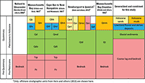 |
Figure 6. Seismic stratigraphic units interpreted by Oldale and Bick (1987), Oldale and Wommack (1987), and Hein and others (2013). Barnhardt and others (2006) published a depth to sediment thickness map, which was used to identify areas of outcropping bedrock on the inner continental shelf between Nahant and Gloucester, Massachusetts. Transgressive (thick red line) and regressive unconformities (dashed red line) were also identified in several of these studies. The stratigraphic unit names and resolution of these studies differed, but the origin and texture of the deposits can be readily combined into a generalized geologic map (fig. 5) to correlate with sediment textures and physiographic zones presented in this study. QbB and QhbC, Holocene beach and bar deposits; QssD, late Pleistocene to Holocene transgressive sand sheet deposits; QsrtD, late Pleistocene to Holocene regressive-transgressive shoreline deposits; QedD, Holocene ebb tidal delta deposits, QocD, late Pleistocene to Holocene offshore coarse deposits; QmB, QhmC, QmmE, and QmscD, late Pleistocene to Holocene offshore marine deposits; QfeB and QhfC, Holocene fluvial and estuarine deposits; QhdC, Holocene deltaic deposits; QdlD, late Pleistocene lowstand delta deposits; QdB and QmdC, Pleistocene glacial-marine deposits; QdoB and QdtC, Pleistocene coarse drift deposits; QtdD and QtE, Pleistocene drumlin till deposits; TcpB,C Tertiary and late Cretaceous coastal plain deposits; Pz B,C, Triassic and older bedrock. |
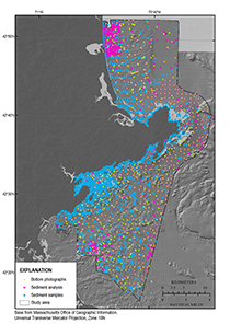 |
Figure 7. Bottom photographs (Barnhardt and others, 2006, 2009; Gutierrez and others, 2000; green dots) and sediment samples collected within the study area and used to aid interpretations. Sediment samples with laboratory analysis are shown as magenta dots, while blue dots are visual descriptions (Ford and Voss, 2010; McMullen and others, 2011; Emily Huntley, Massachusetts Office of Coastal Zone Management, unpub. data, 2012). |
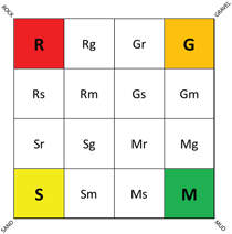 |
Figure 8. Barnhardt and others (1998) bottom-type classification based on four basic sediment units: Rock (R), Gravel (G), Sand (S), and Mud (M). If one of the basic sediment units represents more than 90 percent of the texture, only its uppercase letter is used. Twelve additional two-part units represent combinations of the four basic units, where the primary texture (greater than 50 percent) is given an uppercase letter and the secondary texture (less than 50 percent) is given a lowercase letter. |
 |
Figure 9. Sediment texture polygons were created in ArcGIS by using A, backscatter data, where areas of high backscatter intensity (light tones) have strong acoustic reflections and suggest boulders, gravels, and generally coarse sea-floor sediments ,and areas of low backscatter intensity (dark tones) have weak acoustic reflections and generally are characterized by fine-grained material such as muds and fine sands; B, hillshaded relief imagery, which creates a three-dimensional effect to provide a sense of topographic relief; C, rugosity, where blue polygons outline areas of variation or frequent amplitude changes in topography, often referred to as surface roughness; D, slope, where warm colors represent steeper areas of the map and cool colors represent flatter areas; and E, pseudocolored multibeam backscatter intensity(Butman and others, 2007), which combines backscatter and hillshaded relief. Each data type can provide useful information in a given area when defining texture boundaries. F, Bottom samples and photographs are used to assign a sediment texture within each polygon drawn on the basis of geophysical data and derivatives such as B–E. |
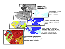 |
Figure 10. Sediment texture and distribution data were mapped qualitatively in ArcGIS by using a hierarchical methodology. Backscatter data were the first input, followed by bathymetry, surficial geologic and shallow stratigraphic interpretations, and photograph and sample databases. DEM, digital elevation model. From Pendleton and others (2013). |
 |
Figure 11. The distribution of sediment textures within the study area from Nahant, Massachusetts, to New Hampshire. The bottom-type classification is from Barnhardt and others (1998) and is based on 16 sediment classes. The classification is based on four sediment units that include gravel (G), mud (M), rock (R), and sand (S) (fig. 8). If the texture is greater than 90 percent, it is labeled with a single letter. If the composition of one component is less than 90 percent, it is labeled with two letters, where the first letter is the primary sediment unit (more than 50 percent) and the second letter is the secondary sediment unit (less than 50 percent). |
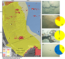 |
Figure 12. Inner continental shelf sediment textures between Cape Ann and New Hampshire with bottom photographs A–D showing sediment texture as defined in select locations. Grain-size statistics are plotted as pie charts showing the relative percentages of gravel, sand, and mud. A, A photograph of the sea floor within an area classified as rock and gravel (Rg). No sample was recovered in this area because of large particle size. B, A photograph of the sea floor within an area classified as primarily sand with some gravel (Sg). C, A photograph from a section of sea floor classified as primarily sand (S). D, A photograph from a section of the sea floor classified as primarily mud with some sand. The viewing frame for photographs A–D is approximately 50 centimeters, and the locations of the photographs are shown as white dots on the sediment texture map. The location of the seismic-reflection profile in figure 17 is also indicated by the black line. Sediment classes are shown in figure 8. %, percent. |
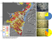 |
Figure 13. Inner continental shelf sediment textures within western Massachusetts Bay with bottom photographs A–D showing sediment texture as it is defined in select locations. Grain-size statistics are plotted as pie charts showing the relative percentages of gravel, sand, and mud. A, A photograph of the sea floor within an area classified as rock (R). No sample was recovered in this area because of large particle size. B, A photograph of a section of sea floor classified as primarily mud with sand (Ms). C, A photograph from a section of sea floor classified as primarily gravel with rock (Gr). No sample was recovered in this area because of large particle size. D, A photograph from a section of the sea floor classified as primarily sand and gravel (Sg) with some mud. This photograph is located near the boundary of a Sg and Gs texture transition. The viewing frame for photographs A–D is approximately 50 centimeters, and the locations of the photographs are shown as white dots on the sediment texture map. The location of the seismic-reflection profile from figure 18 is indicated by the black line. Sediment classes are shown in figure 8. %, percent. |
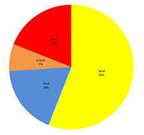 |
Figure 14. Pie chart showing the percentage of each primary sediment unit (texture greater than 50 percent) within the study area. %, percent. |
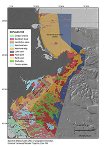 |
Figure 15. The distribution of physiographic zones within the study area from Nahant to Salisbury, including western Massachusetts Bay. The physiographic zone classification is based on Kelley and others (1996) and builds on interpretations developed by Butman and others (2003a,b,c; 2004) and Knebel and Circe (1995), and the zones are delineated on the basis of sea-floor morphology and the dominant texture of surficial material. Areas interpreted by Barnhardt and others (2006, 2009) and Pendleton and others (2013) are shown for regional context and have a slight gray transparency. |
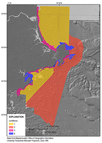 |
Figure 16. Sediment texture regions in the study area and confidence values for data interpretation. Sediment texture polygons are assigned a confidence value from one (highest confidence) to four (lowest) on the basis of the resolution of geophysical data and the number of input data sources. |
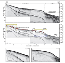 |
Figure 17. A chirp seismic reflection profile across the inner shelf from near the southern end of Plum Island, Massachusetts, to approximately 70 meters (m) water depth (see fig. 12 for profile location). The top panel is the uninterpreted profile, and the middle panel is interpreted to show geologic units. Fluvial and deltaic deposits overlie glacial-marine sediments, which overlie bedrock. The Holocene sand sheet is separated from fluvial sediments by a transgressive unconformity (red line, where the solid line is interpreted and dashed red is inferred). SW, southwest; NE, northeast; V.E., vertical exaggeration. Figure from Barnhardt and others (2009). |
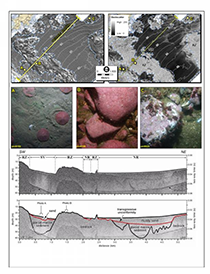 |
Figure 18. Figure showing bathymetry (upper left), backscatter (upper right) with physiographic zone boundaries, and bottom photographs (center) along a seismic reflection profile (bottom two panels). Yellow line on bathymetry panel is the location of the seismic profile (also shown in fig. 13). Shelf valleys formed often between bedrock highs during the lowstand and unconformably overlie glacial-marine deposits. RZ, rocky zone; SV, shelf valley; NR, nearshore ramp; SW, southwest; NE, northeast; m, meters; s, seconds; km, kilometers. From Barnhardt and others (2006). |
|

