


The purpose of these interpretive discussions is to provide a perspective on regional- and national-scale variations in element and mineral distributions in soils and their likely causes. The significant spatial variations shown by most elements and minerals can commonly be attributed to geologic sources in underlying parent materials, but other spatial variations seem clearly related to additional factors such as climate, the age of soils, transported source material, and anthropogenic influences. We attempt to distinguish the influence of these various factors on a regional and national scale. Numerous more local features might similarly be related to these same factors, but these features also have some probability of being an artifact of a random sampling of variable compositions, so that there is some probability of samples with similar compositions occurring in clusters of two or more adjacent sites by chance. Distinguishing such random occurrences from true variability is beyond the scope of the data from which these maps are constructed. Some caution, therefore, is advisable in interpreting the significance of these more local features unless some unique sources or processes can clearly be related to them.
Iron (Fe) is a metallic element used mostly in the manufacture of steel. It is an essential element for all forms of life and is nontoxic. For humans, however, Fe deficiency is a common problem.
Iron is one of the more common elements on Earth, with the abundance in the Earth's upper continental crust estimated to be 3.92 weight percent (wt. %) (Rudnick and Gao, 2003). Ferromagnesian minerals typically occur in ultramafic and mafic igneous and metamorphic rocks, with an average Fe concentration of approximately 9.4 wt. % in ultramafic rocks, and approximately 8.6 wt. % in mafic rocks. Shale is also enriched in Fe with an average concentration of approximately 5.5 wt. %. Other common rock types contain much less Fe with granite averaging about 2 wt. %; sandstone, 1 wt. %; and limestone, 0.5 wt. %. Unconsolidated materials such as alluvial, eolian, or glacial deposits also can have significant Fe concentrations, depending primarily on the source of the deposits.
The distribution of Fe in soils is complex as Fe can be either reduced or oxidized, depending on redox conditions, and the redox state of Fe affects its solubility and distribution in soils, as well as its propensity to form secondary compounds with phosphorus (P), sulfur (S), or carbonate (CO3). Iron in oxidized soils can be released by the weathering of primary ferromagnesian silicate minerals, such as pyroxene, olivine, hornblende, and serpentine. The rapid weathering of ferromagnesian minerals in soils results in a variety of secondary Fe minerals, including Fe oxide (such as hematite) or Fe hydroxide (such as goethite). Released Fe also can bind to organic compounds or be incorporated into sheet silicates (such as chlorite, smectite, and vermiculite), which have a common basal spacing of 14 Å (1 Å (angstrom)= 10-10 meters).
The distribution of mineral resource deposits with Fe as a commodity (major or minor) in the United States, extracted from the U.S. Geological Survey (USGS) Mineral Resource Data System (MRDS) website, can be seen by hovering the mouse here. Statistics and information on the worldwide supply of, demand for, and flow of Fe–bearing materials are available through the USGS National Minerals Information Center (NMIC) website.
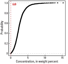
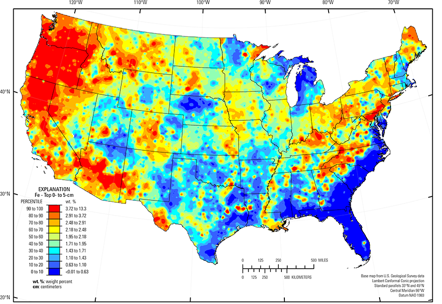
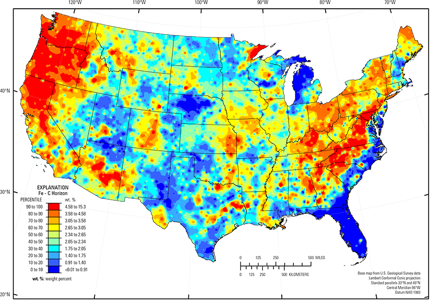
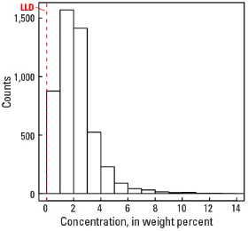
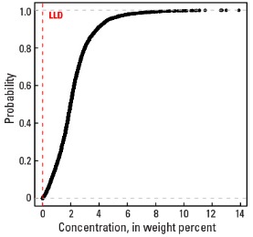
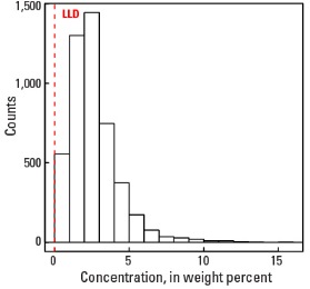
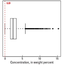
In our data, the median Fe concentration is 2.34 weight percent (wt. %) in the soil C horizon, 1.99 wt. % in the soil A horizon, and 1.95 wt. % in the top 0- to 5-cm layer (see the summary statistics [open in new window]). Nearly all analyzed soils have Fe concentrations above the lower limit of determination (LLD) of 0.01 wt. %. The broad spatial map patterns for Fe among the three sample types are generally similar to one another, but differences exist in the relative concentrations between the soil C horizon and topsoils (soil A horizon and top 0- to 5-cm layer), as suggested by the differences in the median Fe concentrations.
The distribution of elevated concentrations of Fe in the soil C horizon largely reflects the distribution of soil parent materials sourced from ultramafic and mafic rocks or from sedimentary rock and more recent alluvial and eolian, deposits sourced from similar rock types. Examples of such areas include:
- Pacific Northwest and northern California (mafic rocks, including the Columbia River basalts (Swanson and Wright, 1981) and the Cascade Range (basalt);
- Parts of the Central Rocky Mountains and Southern Rocky Mountains (USDA, 2006), and the High Intermountain Valleys (USDA, 2006), of Colorado, Wyoming, Montana, and Idaho (a variety of rock types, including basalt);
- Southern Sierra Nevada Mountains and Carson Basin and Mountains (USDA, 2006), California and Nevada (basalt and andesite);
- Trans–Pecos volcanics (Schruben and others, 1997), Texas (rhyolite, alkalic volcanic rocks, and related alluvium); and
- Mogollon Transition (USDA, 2006), Arizona (basalt and alluvium from mafic volcanics).
In eastern Texas, soils developed on Fe–rich sandstone, siltstone, and claystone (bedrock unit called the Claiborne Group) contain the mineral goethite. In eastern Kansas and western South Dakota, soils with high Fe concentrations formed on shale or alluvium sourced from shale. In the Kentucky Bluegrass area and Nashville Basin (USDA, 2006), soils developed on weathered phosphatic limestone with reported iron–manganese nodules and secondary Fe phosphates. Many of the sample sites with high Fe concentrations through the Gulf and Atlantic Coastal Plain (Fenneman and Johnson, 1946) in Mississippi, Alabama, and Georgia also contain goethite (or hematite), an indication of intense weathering and formation of secondary Fe oxide and hydroxide minerals. Throughout the Piedmont (Fenneman and Johnson, 1946), Fe in soils is likely related to the presence of residual, persistent mafic minerals (such as hornblende) or Fe oxides and hydroxides. Many old, intensely weathered soils in the Piedmont have much higher Fe concentrations in the soil C horizon than in topsoils (soil A horizon and top 0- to 5-cm layer), which is likely due to the occurrence of secondary Fe minerals or the incorporation of released Fe into clay minerals in deeper soil.
The distribution of Fe in soils across the Upper Midwest is controlled by glacial provenance. In this region, melting of glacial ice following late Wisconsinan period advances (16,000 to 12,000 years ago) left the region north of the southern glacial limit (Soller and others, 2012) mantled with a blanket of mixed, immature sediments, from which present–day soils developed. Individual ice lobes (Grimley, 2000) created distinct patterns in soil mineralogy and geochemistry because of varying provenance and ice transport paths. In northeastern and central Minnesota quartz– and feldspar–rich till have a combined local Precambrian basalt and gabbro provenance (Duluth Complex), and a more distant Precambrian crystalline rock/red sandstone provenance. Transported and weathered mafic minerals (such as pyroxene and hornblende) in these glacial sediments contribute Fe to soils. Soils with elevated Fe in eastern Michigan, eastern Indiana, and western Ohio developed on till and other glacial deposits that incorporated black shale.
Areas with relatively low Fe concentrations in soils had no or scarce primary ferromagnesian minerals. Examples include:
- Colorado Plateau (USDA, 2006) (quartz–rich sandstone and eolian sands);
- Central Idaho (granitic rocks);
- Nebraska Sand Hills (USDA, 2006) (soils dominated by quartz and plagioclase feldspar in an area of unconsolidated sand dunes and sheets);
- Southern High Plains (USDA, 2006) of eastern New Mexico and northwestern Texas (quartz–rich eolian and alluvial sediments); and
- Gulf and Atlantic Coastal Plain (Fenneman and Johnson, 1946) (quartz–rich sedimentary rocks and unconsolidated sediments).
The Gulf and Atlantic Coastal Plain (Fenneman and Johnson, 1946) is bisected by the Southern Mississippi River Alluvium and the Southern Mississippi Valley Loess (USDA, 2006). Alluvial sediments have deposited in the Mississippi River valley as the river flooded in recent geologic time. When these sediments dried, winds picked up the fine material and deposited it in thick loess sheets, mainly along the east side of the river valley. The youngest loess sheets are about 10,000 years old. A pattern of higher Fe concentrations in soils developed on these young sediments reflects long–range transport of Fe–bearing materials (likely clays) from the upper part of the Mississippi River drainage basin.
Statistics - 0 TO 5 CM
| Number of samples | 4,841 |
| LLD | 0.01 wt. % |
| Number below LLD | 8 |
| Minimum | <0.01 wt. % |
| 5 percentile | 0.38 wt. % |
| 25 percentile | 1.28 wt. % |
| 50 percentile | 1.95 wt. % |
| 75 percentile | 2.66 wt. % |
| 95 percentile | 4.56 wt. % |
| Maximum | 13.3 wt. % |
| MAD | 1.02 wt. % |
| Robust CV | 52.5% |
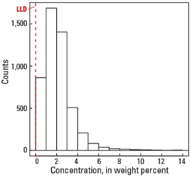
Histogram
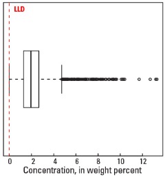
Boxplot
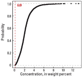
Empirical cumulative distribution function
Statistics - A Horizon
| Number of samples | 4,813 |
| LLD | 0.01 wt. % |
| Number below LLD | 6 |
| Minimum | <0.01 wt. % |
| 5 percentile | 0.36 wt. % |
| 25 percentile | 1.30 wt. % |
| 50 percentile | 1.99 wt. % |
| 75 percentile | 2.75 wt. % |
| 95 percentile | 4.67 wt. % |
| Maximum | 13.9 wt. % |
| MAD | 1.08 wt. % |
| Robust CV | 54.4% |
Histogram
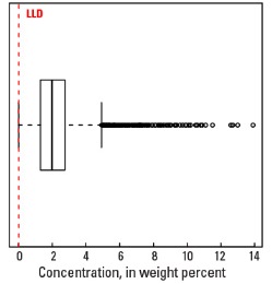
Boxplot
Empirical cumulative distribution function
Statistics - C Horizon
| Number of samples | 4,780 |
| LLD | 0.01 wt. % |
| Number below LLD | 6 |
| Minimum | <0.01 wt. % |
| 5 percentile | 0.53 wt. % |
| 25 percentile | 1.57 wt. % |
| 50 percentile | 2.34 wt. % |
| 75 percentile | 3.28 wt. % |
| 95 percentile | 5.57 wt. % |
| Maximum | 15.30 wt. % |
| MAD | 1.25 wt. % |
| Robust CV | 53.2 % |
Histogram
Boxplot