1 U.S. Geological Survey, Menlo Park, California
2 U.S. Geological Survey, Reston, Virginia
3 U.S. Geological Survey, Portland, Oregon
4 Applied Physics Laboratory, University of Washington, Seattle, Washington
5 U.S. Geological Survey, Vancouver, Washington
6 Geophysical Consulting, Deep River, Connecticut
7 U.S. Geological Survey, Tucson, Arizona
Acoustic Doppler Current Profiler (ADCP)
DATA ANALYSIS AND DATA ARCHIVE
Fig. 1. Data collection site on the San Joaquin River near Vernalis, California. Dual microwave transmitter antennae are shown at upper right attached to the structure that houses radar electronics and the bank-operated cableway controls
Fig. 2. Tethered trimaran-mounted ADCP and BoogieDopp discharge measurement system concurrently measuring vertical velocity profiles. Each instrument transmits data through its own radio-modem operating at a distinct frequency
Fig. 3. Example of ground-penetrating radar (GPR) output. Channel depths at locations corresponding to microwave radar bins are indicated with red Xs
Fig. 4. The physical orientation of the acoustic beams of a BoogieDopp.
Fig. 5. Samples of tow-tank evaluation of BoogieDopp, the towing speeds at 33.4, 66.7, and 91.0 cm/s are shown in solid lines. The velocities measured by the downward looking and forward looking beams are compared with the respective towing speeds
Fig. 6. Comparison of the vertical velocity distributions at Station 6 measured by the BoogieDopp using downward and forward looking beams (with bin size of 11 cm and 4.1 cm), and the velocity distribution measured by an ADCP (with a bin-size of 25 cm). The first velocity measured by the ADCP is 53 cm below surface
Fig. 7. Comparison of the vertical velocity distributions at Station 12 measured by the BoogieDopp using downward and forward looking beams (with bin size of 11 cm and 4.1 cm), and the velocity distribution measured by an ADCP (with a bin-size of 25 cm). The first velocity measured by the ADCP is 53 cm below surface
Fig. 8. Complete velocity distribution in a cross-section of San Joaquin River at Vernalis, California. The velocities were measured on May 17, 2002 using a BoogieDopp. [In this report, depth and velocity are in metric units whereas distance from left bank is in English unit consistent with USGS discharge measurements.]
Fig. 9. Distribution of surface velocity determined by downward and forward beams of a BoogieDopp, and the distribution of the water column mean velocity. [In this report, depth and velocity are in metric units whereas distance from left bank is in English unit consistent with USGS discharge measurements.]
Fig. 10. Near-surface velocity data collected with BoogieDopp contrasted with surface-velocity data collected with microwave radar for selected recording periods on May 17, 2002. [Speed and distance from left bank are in English units consistent with USGS discharge measurements.]
I.1.a_Surface_Velocity_MW_Radar
BDvsRADAR.ppt:
MS PowerPoint (PPT) slides show radar surface speeds plotted with concurrent
BoogieDopp (BD) forward beam, bin 2 (F-2). Indicated times are start time of
the first profile in PDT. The x-axis is distance from left bank, in feet. (Generally
speaking, when the horizontal axis of a plot is distance from riverbank, the
units are in feet regardless of the units used in vertical axis.). The vertical
axis is ft/s.
RadarData.xls:
MS Excel spreadsheet includes radar surface velocity data organized by date
and time (i.e. 517.0747=5/17/02 07:47) with one MS Excel (xls) sheet for each
day of data. There are two rows for each time of data; the 1st row
is along channel and the 2nd row is cross channel
velocity. Units are ft/s. Both distance from the antennae and distance from
the left bank are shown (in feet).
I.1b_Velocity_Profile_ADCP_BD
Date_Time.xls: (14
files). These MS Excel files contain (1) surface velocity information, (2) velocity
profile information (both uncorrected and calibration-corrected BD data, ADCP
data) and (3) the BoogieDopp (BD) ASCII output files generated from the *.dmf
files (dmf files are discharge measurement files generated by the BD). The spreadsheet
labeled surface velocity includes distance depth; BD forward beam velocity,
bin number two (F-2) and downward beam velocity, bin number one (D-1); mean
velocity for profile; and the ratio of mean to surface velocity. There is one
plot of BD surface and mean velocity in each file. These plots do not include
near-surface ADCP data (from bin 1). The first set of data on the velocity profiles
spreadsheet is for BD downward beam; the second data set is for the forward
beam. The BD data columns marked corrected have a calibration factor (determined
in tow tank) applied; units are cm/s. The third data set on the velocity profile
page is the ADCP data. Velocity profile plots (20-21 profile plots, one for
each station in the cross section) have vertical axis converted (with depth)
so that distance below surface becomes distance above bottom (units are cm).
Horizontal axis is speed in cm/s. The third spreadsheet contains the ASCII BD
data as downloaded from hand held computer. Units are m and m/s. Location of
the sample bins (below surface) in meters is shown at end of file.
I.1c_Velocity_Profile_Comps_ADCP_BD
Date_Time.ppt (14 files). These are MS PowerPoint
(PPT) files showing comparisons of ADCP and BD (forward beam and down beam)
measured velocity profiles. Each file has about 20-21 plots, one for each station
across the river. The last plot in each file shows the surface velocities (from
BD F-2 and D-1 beams) and the mean velocity with the calculated ratio (same
as Appendix I.3). The time shown in the last plot is the time of the first profile
as measurements start across the river. Vertical scale is in cm, horizontal
scale is cm/s. The data for these plots are in Velocity_Profile_ADCP_BD.
I.1d_Surface_Velocity_Plots_ADCP_BD
Surface_velocity.ppt:
MS PowerPoint (PPT) plots of BD (F-2 and D-1 bins) and ADCP bin 1. Speeds
for each date and time (PDT) available with profiles at stations across the
river. Units are ft/s and distance from left bank in feet. Times are PDT. There
are 13 plots in the file (4/15 14:58 is not included because there is no concurrent
ADCP data during the BD measurement at 14:58).
Surface_velocity.xls:
MS Excel spreadsheet with uncorrected and corrected velocity from BD
F-2 and D-1 beams in ft/s vs distance (feet) from left bank. Also ADCP Velocity,
bin 1 in cm/s and ft/s vs distance from left bank. There are also plots of BD
(F-2 and D-1 bins) and ADCP bin 1 for each date and time. Velocity data are
in ft/s and distance in feet from left bank. Times are start time (PDT) of measurement
at profile 1. Unlike the surface velocity plots in Appendix .1b (Velocity_Profile_ADCP_BD),
these figures include ADCP measurements from bin 1 and are in ft/s
I.1e_Velocity_Dist_Xsection_Plots_BD
BD_Crosssections.ppt:
MS PowerPoint (PPT) contour plots of river velocity from BD velocity
profiles generated using interpolation and contouring with Matlab software.
There is a separate contour plot from each set of BD measurements. Depth is
given in cm, distance from left bank in feet, and speed in cm/s. Times are the
start times of the first station profiles for discharge measurement in PDT.
I.1f_Water_Velocity_PriceAA
PriceAA_Speed_Q.xls:
MS Excel spreadsheet of Price AA discharge measurement showing Q, measurement
location, and speeds. Units are ft/s and cfs.
I.2_Bathymetry_Measurements
River_Depths_All.xls:
MS Excel spreadsheet 1 contains station depths across the river measured
by ADCP, BD, and GPR. Units are feet for both depth and distance from left bank.
This file also includes individual plots of all ADCP, BD, and GPR station depths
across the river as well as plots of comparisons of the three instruments at
concurrent measurement times.
River_Depths_Comp.ppt:
MS PowerPoint (PPT) graphs of comparisons of depths from the ADCP, BD,
and GPR measurements. Units are in feet for depth and distance in feet from
left bank. Times for each plot are time (PDT) of the first measurement (profile)
in the set for the river cross section.
I.3_Mean_to_Surface_Velocity
Ratio_Mean_Surface.ppt:
plots are the same as the last plot in each file shown in directory
Velocity_Profile_Comps_ADCP_BD. These show surface
velocities measured by BD F-2 and D-1 beams only; no ADCP data are displayed.
Plots show surface and mean velocity with the calculated ratio. The time shown
in the plot is the time of the first profile as measurements start across the
river. Units for vertical scale is cm and horizontal scale is cm/s. The data
for these plots are in Velocity_Profile_Comps_ADCP_BD.
I.4a_River_Discharge_Vernalis_Gage
Vernalis.11303500
: Provisional discharge data at Vernalis gage site in standard USGS data
format.
I.4b_River_Discharge_all
Discharge.ppt
: MS PowerPoint (PPT) slide include plots of (1) corrected BD vs ADCP, (2) BD
measured and calculated, ADCP Price AA, and Radar with GPR, and (3) regression
of calculated and measured BD Q.
Discharge_Data.xls
: MS Excel spreadsheet with all discharge data including ADCP (individual and
averaged) BD, and Radar with GPR. Times are PDT. Spreadsheet includes comparison
plots of all data and BD vs ADCP.
I.5a_BoogieDopp_Stennis_TowTank
Stennis.xls:
MS Excel spreadsheet shows summary of BD tests including tow carriage
speeds (ft/s) and BD results (ft/s and cm/s) for tow carriage tests in tow tank.
| Multiply | By | To obtain |
|---|---|---|
|
inch (in.) |
2.54 | centimeter (cm) |
|
foot (ft) |
0.3048 | meter (m) |
|
mile (mi) |
1.609 | kilometer (km) |
|
square mile (mi2) |
2.590 | square kilometer (km2) |
|
cubic foot per second (ft3/s) |
0.02832 | cubic meter per second (m3/s) |
| centimeter (cm) |
0.3937 |
inch (in.) |
| meter (m) |
3.281 |
foot (ft) |
|
kilometer (km) |
0.6214 | mile (mi) |
|
square kilometer (km2) |
0.3861 | square mile (mi2) |
|
cubic meter per second (m3/s) |
35.31 | cubic foot per second (ft3/s) |
Specific conductance is given in microsiemens per centimeter at 25 degrees Celsius (µS/cm at 25°C).
|
ADCP BD Deg. GHz GPR GPS KHz MHz MS NGVD PDT USGS VAMP |
Acoustic Doppler current profiler BoogieDopp discharge measurement system Degrees GigaHertz Ground penetrating radar Global positioning system KiloHertz MegaHertz Microsoft National Geodetic Vertical Datum Pacific daylight time United States Geological Survey Vernalis Adaptive Management Program |
Accurate measurement of flow in the San Joaquin River at Vernalis, California, is vital to a wide range of Federal and State agencies, environmental interests, and water contractors. The U.S. Geological Survey uses a conventional stage-discharge rating technique to determine flows at Vernalis. Since the flood of January 1997, the channel has scoured and filled as much as 20 feet in some sections near the measurement site resulting in an unstable stage-discharge rating. In response to recent advances in measurement techniques and the need for more accurate measurement methods, the Geological Survey has undertaken a technology demonstration project to develop and deploy a radar-based streamflow measuring system on the bank of the San Joaquin River at Vernalis, California. The proposed flow-measurement system consists of a ground-penetrating radar system for mapping channel geometries, a microwave radar system for measuring surface velocities, and other necessary infrastructure. Cross-section information derived from ground penetrating radar provided depths similar to those measured by other instruments during the study. Likewise, surface-velocity patterns and magnitudes measured by the pulsed Doppler radar system are consistent with near surface current measurements derived from acoustic velocity instruments. Since the ratio of surface velocity to mean velocity falls to within a small range of theoretical value, using surface velocity as an index velocity to compute river discharge is feasable. Ultimately, the non-contact radar system may be used to make continuous, near-real-time flow measurements during high and medium flows. This report documents the data collected between April 14, 2002 and May 17, 2002 for the purposes of testing this radar based system. Further analyses of the data collected during this field effort will lead to further development and improvement of the system.
Accurate measurement of flow in the San Joaquin River at Vernalis, California, is vital to a wide range of Federal and State agencies, environmental interests, and water contractors. Streamflow data are used in managing reservoir releases, preparing river and estuary flow forecasts, and scheduling water withdrawals for the Federal and California State Water Project canals for delivery to users in central and southern California. Every year from approximately April 15 to May 15, the gage on the San Joaquin River at Vernalis is the principal measurement location for determining flow variations during the Vernalis Adaptive Management Program (VAMP). The VAMP is a joint program carried out by the U.S. Bureau of Reclamation, the California Department of Water Resources, and water contractors to improve the survivability of outward migrating juvenile Chinook salmon by temporarily increasing releases from upstream water-supply reservoirs, constructing flow and fish barriers on some downstream tributaries, and reducing pumping operations at the Federal and California State Water Project intakes. During the VAMP, the need for accurate, near-real-time flow data increases and the Vernalis streamflow records come under close scrunity.
Conventional streamgaging techniques employed by the U.S. Geological Survey (USGS) rely on periodic physical measurements of water velocities and channel widths and depths to measure flow, and stage-discharge relations (ratings) to relate the measured flow to stream stage. Continuous, real-time flow records are developed by applying these ratings, along with periodic corrections, to stage readings. The stage-discharge process is reliable and accurate only if the relationship between stage and discharge is known; otherwise, changes in channel geometry, bed slope, and roughness may result in significant changes in the rating (shifts). At Vernalis, bedforms vary with time (altering channel geometries and roughness) resulting in unpredictable rating shifts. These uncertainties lead to shift estimates giving rise to inaccurate estimates of the river discharge.
Although measuring river discharge is always an important task in water resources management, present measurement practices are labor intensive and often expose field technicians to potential hazards. Although there are significant technical hurdles that must be overcome, some developing technologies are emerging that could replace or supplement conventional streamgaging methods within the USGS (Mason and others, 1992). With these objectives in mind, the Hydro 21 committee was established and charged with the mission of investigating new and advanced technologies that might change the paradigm of streamgaging within the USGS (Cheng and others, 2002). For a number of reasons, most importantly concerns for the safety of those making the measurements, the Hydro-21 committee chose a non-contact approach for determining river discharge (Costa and others, 2000). The committee has been experimenting with adapting ground-penetrating radar (GPR) for measuring channel cross-section (Spicer and others, 1997) and microwave or high frequency (HF) radars to measure surface velocity distribution. Following this development, it is believed that water surface velocity can be used as an index velocity with which the water column mean-velocity can be estimated for computing river discharge. In 1999, radar-based systems were successfully deployed by the USGS in an experiment to test the concept of non-contact measurement of streamflow at the Skagit River in Washington (Costa and others, 2000).
The radar based streamflow system has demonstrated the potential for application to unstable alluvial channels such as the San Joaquin River at Vernalis, California (to be referred to as Vernalis in the remainder of this report). To further evaluate and develop the radar-based streamflow technology, the USGS undertook a measurement program at Vernalis in water year 2002. The objective of the program was to collect detailed hydrological data in support of further evaluation of a radar-based, non-contact flow measurement system at Vernalis during the 2002 VAMP experiment. Ultimately, the radar system could be used for continuous, near-real- time flow measurements during high and medium flows. To support these efforts, a variety of conventional instruments were used in conjunction with the radar system to make measurements of flow and channel cross-section, at Vernalis from April 14 to May 17, 2002.
This report documents field data collected in the San Joaquin River at Vernalis during the 2002 VAMP program. In the following sections, a short description of the experimental site is given, followed by a summary of the data collection methods. The methods of data reduction and analysis for each instrument are also presented. A discussion and conclusion section and appendices with data sets are included at the end of this report. All collected data are archived and available so that original data can be used for research and further analysis.
The authors wish to thank Bill Brazelton, Joe Grant, Joe Cruz, Mike Galvez, Neil Ganju, and Kevin Wright of the USGS California District for their efforts in the collection and interpretation of the field data. This project was funded by the USGS National Streamflow Information Program, National Research Program, and Hydro 21 Program, and by the CALFED Bay-Delta Authority administered by the U.S. Environmental Protection Agency.
The USGS has an established streamgaging station (11303500) for the San Joaquin River near Vernalis, California (Vernalis). The station is located at 37°40'34" latitude and 121°15'55" longitude in El Pescadero Grant, San Joaquin County on the west or left (looking downstream) bank of San Joaquin River 12 ft (3.7 m) downstream from Durham Ferry Highway Bridge. The site is 2.6 mi (4.2 km) downstream from the Stanislaus River, and 3.2 mi (5.2 km) northeast of Vernalis, California. The drainage area is about 13,536 mi2 (35,058 km2) including about 2100 mi2 (5439 km2) in James Bypass. The water discharge record was first established in July 1922, and continues to the present (2002). The gage height record is obtained with a nitrogen bubbler gage system; the gage datum is the National Geodetic Vertical Datum, 1929 (NGVD 1929). Records at this station are generally good. During low flow conditions, the river consists mainly of the return flows from irrigation areas. The maximum recorded-discharge at the site was 79,000 f3/s (2237 m3/s) on December 9, 1950. Water level was at 32.81 ft (10.00 m) at that time. The maximum recorded-elevation was 34.88 ft (10.63 m) on January 5, 1997.
During the 2002 VAMP experiment, the Hydro-21 Committee occupied a study site which was located in a straight stretch of the San Joaquin River approximately 1300 ft (400 m) downstream from the USGS gaging station at Vernalis. There is no tributary, or over-bank flow or storage between the gaging station and the study site, thus the river discharge determined at the gaging station should be the same as the discharge measured at the study site. A flat area on the left (west) river-bank provided space for equipment and instrument staging. At the study site, the river was approximately 230 ft (70 m) wide. The maximum depth was about 7 ft (2.1 m), with an averaged depth of 3.5 ft (1.1 m).
The river channel is asymmetric with the maximum water depth located closer to the left (west) bank. A temporary structure was built on the left bank to house a bank-operated cableway. The cableway was used to position measurement instruments over or on the river for flow, velocity, and water depth measurements.
The radar-based streamgaging system included a GPR for mapping channel geometries and a microwave radar system for measuring water-surface velocities. Due to site access restrictions, permanent electrical service was not installed. Consequently, the radar systems could only be run on an intermittent basis with electrical generators until May 7, 2002 when tempoary service was provided. After May 7, 2002 the microwave radar was operated continuously. However, on several days, high temperatures affected the radar processing unit, resulting in some periods of lost record. The microwave radar was installed on April 14, 2002 (fig. 1). The radar was activated during daylight hours from April 15 to April 18, 2002. Thereafter, it was used to make near-continuous measurements of surface velocities on April 24, May 1, and May 7 through May 17, 2002.
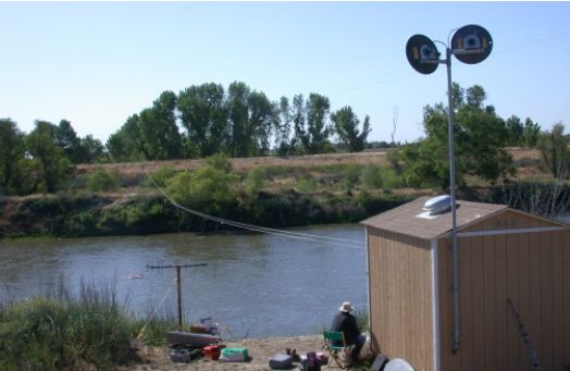 |
| Fig. 1. Data collection site on the San Joaquin River near Vernalis, California. Dual microwave transmitter antennae are shown at upper right attached to the structure that houses radar electronics and the bank-operated cableway controls. |
To evaluate radar measured surface-velocity, intensive surveys of velocity profiles were conducted. Velocity profiles were measured using various Acoustic Doppler Current Profilers (ADCPs) (RDI 600 KHz Workhorse1, RDI 1200 KHz Workhorse with a ZedHed transducer, and RDI 1200 KHz Rio Grande with a ZedHed and radio modem), a conventional Price AA current meter, and a BoogieDopp (BD) discharge measurement system manufactured by Nortek.
Different instruments were tested to identify an instrument that could collect accurate near-surface velocities and function in relatively shallow waters at Vernalis.
To achieve a better understanding the river hydraulics, velocity distributions in the complete river cross-section were measured by an ADCP and a BD (Cheng and Gartner, 2003). Typically, two or more pieces of equipment were paired (fig. 2) and positioned at 20-21 fixed measurement locations across the river using the bank-operated cableway. Velocity data were logged at each measurement location as detailed below. By integrating the detailed velocity profile measurements in the river cross-section, the river discharge was computed. In addition to the velocity measurements, moving-boat discharge measurements were made using ADCPs attached to and transported by the cableway for comparison with other independent discharge measurements. Depths determined by acoustic instruments and sounding weight were periodically verified by an Eagle Mark 1 model fathometer.
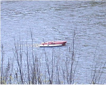 |
Fig. 2. Tethered trimaran-mounted ADCP and BoogieDopp discharge measurement system concurrently measuring vertical velocity profiles. Each instrument transmits data through its own radio-modem operating at a distinct frequency. |
1 Any use of trade, firm, or product names is for descriptive purposes only and does not imply endorsement by the U.S. Government.
Water surface velocity was measured by a pulsed Doppler radar operating in the X-band (microwave). The radar, developed at the University of Washington, emits bursts of 9.36 GHz microwaves across the water surface from the left riverbank. The location of the radar “range cell” was determined by time-gating (sampling the reflected radar signals at time intervals corresponding to discrete ranges). The Bragg scatter reflected from waves moving toward or away from the radar is shifted slightly in frequency by the current (Doppler shift) (Paduan and Graber, 1997). The magnitude of this frequency shift is directly proportional to the velocity of water at the “range cell”. Frequency shift data are collected and averaged over a 30.5-second interval.
To determine the downstream and cross-stream velocity components, two microwave antennas are used, one transmitting and receiving a signal 23 degrees upstream, and another transmitting and receiving a signal 23 degrees downstream of the measurement section. The Doppler-shifted radar signals along the beam directions are collected and grouped into bins, each approximately 12.3 ft (3.75 m) long. The width of a range cell varies with distance from the antennae; the width varied from about 2.6 ft (0.8 m) near the left bank to about 12.5 ft (3.8 m) at the right (far) bank. Thus, the raw radar data represent averaged line-of-sight velocities in a range cell of varying width rather than point velocities at the measurement stations. Furthermore, the distance between the upstream and downstream range cells varies from 14.4 m at the left bank to 70.4 m at the far (right) bank. For the technique to produce accurate velocity measurements, the average surface velocity must be assumed to be constant over these distances. This assumption might have important implications when interpreting the velocity data for comparison with other independent flow measurements.
GPR units emit radar waves that pass through or are reflected by media to varying degrees depending upon whether the medium is air, water, or soil. The intensity of the reflected signal is primarily a function of the electromagnetic impedance of the media. The GPR measures the elapsed time between the emission of a transmitting radar signal and the arrival of its reflection to estimate the distance to the signal reflectors. At the interface where the impedance of the media changes, a distinct echo can be detected. Based on this principle, GPR can be used to determine the location of air-water and water-soil (river bed) interfaces. When a GPR is towed across a river, a continuous record of the location of the interface is obtained. A Mala Geoscience Ramac X3M GPR system with a 100 MHz shielded antenna was used during the Vernalis experiment. This GPR is a pre-production model and is among the first of its kind released for field use. A conversion factor of 0.11 ft/ns (nanosecond) (0.03 m/ns) was assumed to convert the GPR data (speed of electro-magnetic wave in water) to estimates of channel depth. The GPR was suspended from the bank-operated cableway (fig. 1) and transported across the river at 2 to 4 ft (0.6 to 1.2 m) above the water surface. A shaft encoder attached to the suspension hoist tracked the horizontal position of the GPR. An example of GPR data following post-processing is shown in figure 3. The distance between the air-water and water-soil interfaces is the water depth of the river channel. Channel depths at locations corresponding to the microwave radar bins are indicated on figure 3.
The accuracy of GPR measurements is adversely affected by high conductivity of water. Water conductivity of about 1000 S/cm (microsiemens per centimeter) is sufficient to preclude reflection of any usable radar signal. During dry periods the water in the San Joaquin River consists largely of irrigation returns; conductivity is generally greater than 500 S/cm during those periods of the year. During the VAMP experiment, the conductivity of San Joaquin River water was expected to be low due to flows from reservoirs and snowmelt. However, in 2002, mean flows for April and May were about half of their normal values. Conductivity values during the experiment ranged from a high of 850 to a low of about 260 S/cm resulting in degraded GPR performance when conductivity was high.
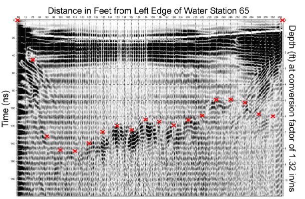 |
| Fig. 3. Example of ground-penetrating radar (GPR) output. Channel depths at locations corresponding to microwave radar bins are indicated with red X s. |
An ADCP determines water velocity profiles by transmitting sound pulses at a fixed frequency and measuring the frequency (or phase) shift in acoustic echoes reflected back from scatterers in the water (Simpson, 2001). It can be deployed with the acoustic beams pointing vertically up or pointing vertically down. In this study, the ADCP was mounted in the middle of a small trimaran with the transducers oriented down and just submerged below the water surface (fig. 2). The trimaran was tethered to the cableway; by controlling the movements of the cable, the trimaran could be towed across the river to replicate a traditional moving-boat ADCP discharge measurement or could be kept stationary for velocity profile measurements. There are several modes of ADCP operation that could be selected for these measurements depending upon the water depth and other considerations. An evaluation and detailed discussion of the ADCP modes can be found in Gartner and Ganju (2002). Typically, the highest sampling rate and smallest usable bin-size were chosen to give maximum spatial resolution of velocity distribution. Utilizing a 25 cm bin size and appropriate blank distance, the first velocity (bin) measured by a 1200 KHz ADCP was at about 50 cm below water surface. Each single-ping velocity measurement was saved; these high frequency velocity data could be used for further analysis of the turbulence properties of the flow in the water column. Because of local water depth and flow conditions, RDI-mode-1 was generally used for the ADCP fixed station measurements, which included more than 400 single-ping samples. The entire procedure took about 3 minutes per station to complete.
The BoogieDopp (BD) is a fairly new acoustic instrument designed for river discharge measurements in small and shallow rivers. The tethered system consists of a Nortek Aquadopp current profiler mounted on a short boat similar to a boogie board which orients itself in the direction of the moving stream (Gordon and Marsden, 2002). The BD assumes the direction of the flow (for the entire water column) is the same as the longitudinal axis of the BD during the measurement.
The instrument operates in a mode similar to a narrow band ADCP. BD has three acoustic beams operating at 2 MHz. Two vertical beams point downward at 25o angle forward and aft from the vertical, and a third beam points forward at 20o from the horizontal (fig. 4). If the bin size of the downward looking beams is set to 11 cm; considering the blanking distance, the first velocity measurement is estimated to be at about 21 cm below free-surface. Although the bin-size of the forward beam is also 11 cm, the equivalent vertical resolution is 4.1 cm. Thus, the orientation of the forward beam is designed to measure velocity in a surface layer of the water column in high vertical resolution.
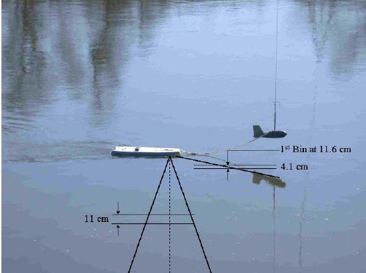 |
| Fig. 4. The physical orientation of the acoustic beams of a BoogieDopp. |
Prior to this study BD was evaluated in a tow tank at the U. S. Geological Survey’s Hydraulics Test Facility at Stennis Space Center, Mississippi (Cheng and Gartner, 2003). Based on the tow tank evaluation, a constant correction factor of 10.6 percent and 17 percent was applied to the velocities produced by the downward and forward looking beams using the beta-version of the BD firmware. (Recent firmware modifications have eliminated use of large correction factors in production versions of the BD.) After applying correction factors, errors in measured velocities are expected to be within 3 percent for the downward beams, and 4 percent for the forward beam. The measured velocity in the first bin of the forward beam was typically biased ~15 percent low during tow tank experiments, thus the measured velocity in the first bin is not used in field applications (fig. 5). The velocity in the second bin, which is located at about 11 cm below the water surface, is considered the first valid measurement.
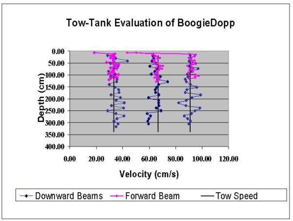 |
| Fig. 5. Samples of tow-tank evaluation of BoogieDopp, the towing speeds at 33.4, 66.7, and 91.0 cm/s are shown in solid lines. The velocities measured by the downward looking and forward looking beams are compared with the respective towing speeds. |
The basic data collected during the VAMP program were pre-processed and converted to engineering units. Pre-processing of these data was usually carried out using the firmware provided by the respective instrument manufacturers. Basic data include the velocity profiles collected by ADCP and by BD; water surface velocity distribution measured by radar; surface velocity measured by Price AA current meter; water depth and channel cross-section determined by GPR, ADCP, BD, and fathometer; and discharge measured by BD and ADCP. Table 1 summarizes the frequency and time and dates of data collection by these instruments; the basic data are archived in the appendices included with this report.
Table 1. The dates and times of basic data collection between April 14, 2002 and May 17, 2002. The type of data and instrument used are given in the first row.
| DATE | Number of BD Q and Profiles |
BD Start/Stop Time (PST) | Number of ZedHed ADCP Profiles | Number of 600 kHz WH Profiles | Number of Averaged ADCP Q | Number of Price AA Q at USGS Gage | Time of GPR Depth | Time of Fathometer Depth |
|---|---|---|---|---|---|---|---|---|
| 4/14/2002 | 1 |
|||||||
| 4/15/2002 | 2 |
12:00-13:20 13:56-15:03 |
1 |
1 |
18:31 |
16:00, 18:13 |
||
| 4/16/2002 | 2 |
9:38-10:55 13:04-14:27 |
2 |
4 |
09:40, 15:55 |
13:15, 16:35 |
||
| 4/17/2002 | 1 |
8:57-10:21 |
1 |
3 |
1 |
09:40, 11:40, 13:55, 16:30 |
14:45 |
|
| 4/18/2002 | 1 |
9:25 |
||||||
| 4/24/2002 | 1 |
12:14-13:45 |
1 |
2 |
1 |
12:34, 15:38 |
||
| 5/1/2002 | 1 |
1 |
11:45 |
|||||
| 5/7/2002 | 1 |
12:10-13:21 |
1 |
2 |
||||
| 5/8/2002 | 2 |
7:47-9:03 12:11-13:25 |
2 |
3 |
1 |
11:10, 15:15 |
||
| 5/10/2002 | 11:40, 15:35 |
14:50 |
||||||
| 5/15/2002 | 2 |
9:42-10:59 13:07-14:28 |
2 |
3 |
1 |
08:25 12:25, 15:55 |
09:30 13:45 |
|
| 5/16/2002 | 2 |
8:33-9:51 13:36-14:53 |
2 |
6 |
1 |
08:00, 16:55 |
||
| 5/17/2002 | 1 |
9:01-10:18 |
1 |
4 |
1 |
08:05, 11:35 |
13:00 |
As an example of the vertical velocity distributions measured by ADCP, and by the downward and forward pointing acoustic beams of the BD, measurements made on May 17, 2002 at 65 ft (19.8 m) from the left bank are shown in figure 6. Measured velocities by ADCP and BD are in good general agreement when data are available for comparison. The forward beam of the BD measures the velocity closest to the water surface and provides the finest vertical resolution. The velocity distributions in the over-lapping region measured by the forward looking beam and downward looking beams of the BD are in very close agreement, but the vertical spatial resolution in the downward beam (11 cm) is nearly three times the size the forward beam (4.1 cm).
Clearly, under these flow conditions and instrument setup requirements, the ADCP is limited in its ability to measure velocity near the free surface. Furthermore, the vertical spatial resolution is relatively coarse (25 cm). The velocity profile determined by the ADCP shows smaller velocity gradient (shear) than the BD measurements; this could be the result of coarse spatial resolution and spatial averaging of velocities. The measured velocity distribution by the BD in the surface layer suggests that a maximum velocity exists below the free surface. Since wind was weak during the time of the measurements, the probable cause of the maximum velocity below the free-surface is the presence of secondary circulation. This station is close to the left bank and near the location where the water is deepest in the cross-section. The geometry of the channel cross-section is conducive for the development of secondary flow. The presence of secondary circulation is more evident in the composite display of velocity distribution in the river cross-section.
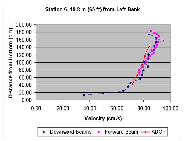 |
| Fig. 6. Comparison of the vertical velocity distributions at Station 6 measured by the BoogieDopp using downward and forward looking beams (with bin size of 11 cm and 4.1 cm), and the velocity distribution measured by an ADCP (with a bin-size of 25 cm). The first velocity measured by the ADCP is 53 cm below surface. |
Similar comparisons of the velocity profiles measured at 125 ft (38.1 m) from the left bank are shown in figure 7. The effect of secondary flow is evident at this station (also see fig. 8 for the velocity distribution in the river cross-section). Since the ADCP cannot reliably measure velocity within about 50 cm of the free surface, the important properties of velocity distribution near the surface cannot be detected. This is most critical in shallow water where unmeasured regions near the surface and near the bottom make up a larger percentage of the total water column. Thus, it is important to use only the appropriate measuring device if the velocity properties in the region near the free surface are to be resolved.
Twenty-one vertical velocity profiles measured by the BD on May 17, 2002 are combined to give a composite plot showing the complete 2-D velocity distribution in a river cross-section in figure 8. The river channel is asymmetric with deeper channel near the left bank. Near the water surface and water-sediment boundaries, the velocity is not measured. These ‘blanked out’ regions are much reduced in the case of the BD. The overall velocity properties are clearly depicted in the cross-sectional plot of velocity distribution. The consistent presence of a maximum velocity core, which is located near the left bank of the river, was possibly due to the presence of secondary flows and the channel geometry.
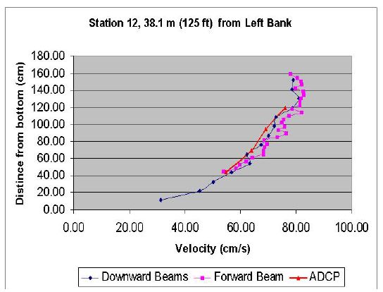 |
| Fig. 7. Comparison of the vertical velocity distributions at Station 12 measured by the BoogieDopp using downward and forward looking beams (with bin size of 11 cm and 4.1 cm), and the velocity distribution measured by an ADCP (with a bin-size of 25 cm). The first velocity measured by the ADCP is 53 cm below surface. |
Based on the velocity profiles measured by the BD, the water column mean velocity is computed for all data sets (appendix I.1b). As an example (May 17, 2002), the mean velocities are plotted against the surface velocities measured in the first bin of the downward beams and the second bin of the forward-looking beam (fig. 9). This type of data are archived in appendix I.3. It is interesting to note that the independently measured surface velocities are in very close agreement except at two stations. The cause of the discrepancy at these stations is not known. If the velocity profile follows the log-law-of-the-wall (Chow, 1959), the theoretical ratio of mean velocity over surface velocity is 0.85. The measured ratio varies between 0.80 and 0.93. The higher values are found near the core of high velocity where maximum velocity is located below the water surface. In this region, the velocity in the near surface layer does not follow the log- law-of-the-wall. In contrast, low-ratio values are found in shallow regions where maximum velocity is found at near free surface, and the velocity distribution is closely approximated by the log-law-of-the-wall. For velocity data collected on May 17, 2002, the mean value for the mean to surface velocity ratio is 0.88, which is reasonably close to the theoretical value of 0.85. For all data sets, the cross-sectional average of the mean to surface velocity ratio is 0.88 with a range from 0.84 to 0.91 (appendix_I.3).
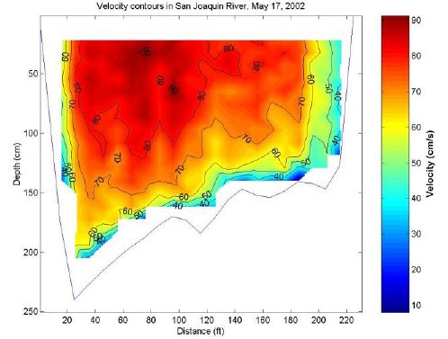 |
Fig. 8. Complete velocity distribution in a cross-section of San Joaquin River at Vernalis, California. The velocities were measured on May 17, 2002 using a BoogieDopp. [In this report, depth and velocity are in metric units whereas distance from left bank is in English unit consistent with USGS discharge measurements.] |
 |
| Fig. 9. Distribution of surface velocity determined by downward and forward beams of a BoogieDopp, and the distribution of the water column mean velocity. [In this report, depth and velocity are in metric units whereas distance from left bank is in English unit consistent with USGS discharge measurements.] |
The ADCP and BD were towed across the river cross-section using the cableway to provide a series of discharge measurements (appendix I.4b). An averaged value of 70.2 cms (cubic meters per second) (2476 cfs) was determined by ADCP on May 17, 2002. The corresponding BD discharge measurement based on the firmware was 76.85 cms (2712 cfs). The discharge computed from the measured surface velocities as index is 75.32 cms (2658 cfs). During the ADCP discharge measurements, there were some movements of the river bed detected by the bottom tracking measurements (GPS position information was not available). The effects of a moving bottom are not removed from the ADCP discharge measurements, thus the reported river discharge is biased low. With this consideration, the ADCP and BD discharge measurements are in reasonable agreement. Thus these results imply that the surface water velocity could be used as the index for computing river discharge. Results from all discharge measurements (ADCP, BD, Price AA, and radar) are archived and documented in appendix I.4b.
This report documents field data collected in the San Joaquin River at Vernalis during the 2002 VAMP program. A short description of the experimental site and a summary of the characteristics of instruments used and deployment methods are presented. The methods of data reduction and analysis for each instrument is also provided. All collected data are archived and available in Appendices so that others can use these original data for research and further analysis.
The main objective of this report is to document all the basic data collected during the field experiment. Final data analysis is incomplete, but preliminary results indicate the surface- velocity patterns and magnitudes collected by the pulsed Doppler radar system are very similar to surface-velocity patterns and values derived from extrapolation of acoustic instrument results. For example, surface-velocity data collected with the microwave radar for various recording periods on May 17, 2002 are compared with near-surface velocity data collected with BoogieDopp in figure 10. The discharge (determined by stage-discharge relation) during this measurement period decreased slightly from 68.10 cms (2400 cfs) to 67.15 cms (2360 cfs). Overall, the radar data are very consistent with BD velocity observations. Velocity data recorded by BD between 10:00 and 11:18 are generally within 0.2 ft/s (5 cm/s) of surface-velocity data collected by radar at 10:33 except at station 40 ft (12 m) from the left bank where the radar measured speed is about 0.75 ft/s less than that measured by BD. Otherwise, there does not appear to be a clear bias in the surface velocities relative to and BD data (collected at 13 cm below the water surface). Some discrepancies may be due to the difference in depth where the velocities were measured. Another reason could be the longitudinal separation of radar measurement locations. Due to the angle between the transceivers and the width of the river, the radar data represent average velocities over lengths of the river from 21 to as much as 113 feet (6.4 to 34.4 m) either side of the cableway. Velocities measured by BoogieDopp are the velocities for the river along the cableway.
GPR-derived channel cross-sections were difficult to derive in high-conductivity waters of the San Joaquin River near Vernalis, California. Nevertheless, preliminary results indicate GPR-derived cross-sections were very similar to depths measured with a fathometer (appendix I.2).
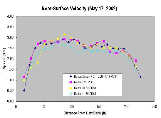 |
| Fig. 10. Near-surface velocity data collected with BoogieDopp contrasted with surface-velocity data collected with microwave radar for selected recording periods on May 17, 2002. [Speed and distance from left bank are in English units consistent with USGS discharge measurements.] |
River hydraulics is quite complex in natural channels and rivers. For practical and engineering purposes, the flows in river channel are often characterized by depth averaged or cross-sectionally averaged properties. While these simplifications might be justifiable and necessary for practical reasons, it is important to be cognizant about the complex nature of the three-dimensional free-surface flows in rivers and open channels. A better understanding of the hydraulic properties in natural rivers would give rise to a more accurate approximation in practical applications. In this study, the velocity distribution in a river cross-section has been investigated in detail. The complete velocity distribution in the river cross-section was measured by a BD, an instrument that is capable of measuring water velocity starting at 11 cm below the water surface. The downward and forward acoustic beam systems give vertical velocity resolution at 11 cm and 4.1 cm, respectively. The velocity profiles measured by BD and the composite velocity distribution determined from those profiles show a maximum velocity core below the free surface near the left bank where the water is deepest. Revealing this detailed velocity distribution is possible because the BD is capable of measuring the velocity in the near surface layer.
Recent advances in measurement techniques have suggested the use of remotely measured surface velocity to determine river discharge. The validity of this approach hinges upon, in part, a stable relationship between the water column mean velocity and the surface velocity. Using the detailed velocity profiles measured in this study, the computed mean velocity to surface velocity ratio is in the range of 0.80 and 0.93 with a mean value of 0.88, while the theoretical value is 0.85. Since the velocity ratio falls in a small range, using surface velocity as index to compute the river discharge would probably not be a major source of error. This conclusion is only based on a small sample of measurements from this study and from measurements at a few other sites not discussed in this report; it is recommended that detailed velocity distribution be measured in rivers with a wide range of width to depth ratio, a variety of bed roughness and bed material, and for high flow and low flow regimes. A conclusive assessment of the appropriate choice of the mean to surface velocity ratio for the computation of river discharge is only possible after examining a sufficiently large number of case studies.
Cheng, R. T., J. E. Costa, F. P. Haeni, N. B. Melcher, and E. M. Thurman, 2002, In search of technologies for monitoring river discharge, in Advances in Water Monitoring Research, T. Younos, Ed., Water Resources Publications, p. 203-219.
Cheng, R. T. and J. W. Gartner, 2003, Complete velocity distribution in river cross-sections measured by acoustic instruments, Proceedings of the IEEE Seventh Working Conference on Current Measurement, San Diego, CA, March 13-15, 2003, pp. 21-26.
Chow, V. T., 1959, Open Channel Hydraulics, McGraw Hill, 680 p. Costa, J. E., K. R. Spicer, and R. T. Cheng, F. P. Haeni, N. B. Melcher, and E. M. Thurman, 2000, Measuring stream discharge by non-contact methods: A proof-of-concept experiment: Geophysical Research Letters, Vol. 27, No. 4, Feb. 2000, pp. 553-556.
Costa, J. E., K. R. Spicer, and R. T. Cheng, F. P. Haeni, N. B. Melcher, and E. M. Thurman, 2000, Measuring stream discharge by non-contact methods: A proof-of-concept experiment: Geophysical Research Letters, Vol. 27, No. 4, Feb. 2000, pp. 553-556.
Gartner, J. W. and N. K. Ganju, 2002, A preliminary evaluation of near transducer velocities collected with low-blank acoustic Doppler current profiler, Proceedings, ASCE 2002 Hydraulic Measurements and Experimental Methods Conference, Estes Park, CO, July 2002, published as CD without page numbers.
Gordon, Lee and Randy Marsden, 2002, The BoogieDopp: a new instrument for measuring discharge in small rivers and channels, Proceedings, ASCE 2002 Hydraulic Measurements and Experimental Methods Conference, Estes Park, CO, July 2002, published as CD without page numbers.
Mason, R. R., J. E. Costa, R. T. Cheng, K. R. Spicer, F. P. Haeni, N. B. Melcher, W. J. Plant, W. C. Keller, and Ken. Hayes, A proposed radar-based streamflow measurement system for the San Jaoquin River at Vernalis, California, Proceedings, ASCE 2002 Hydraulic Measurements and Experimental Methods Conference, Estes Park, CO, July 2002, published as CD without page numbers.
Paduan, J. D. and H. C. Garber, 1997, Introduction to high-frequency radar: reality and myth, Oceanography 10: 36-39.
Simpson, M. R. and R. N. Oltmann, 1992, Discharge-measurement system using an acoustic Doppler current profiler, USGS Water Supply Paper 2395, 34 p.
Simpson, M. R., 2001, Discharge measurements using a broad-band acoustic Doppler current profiler, USGS Open-File Report 01-1, 123 p.
Spicer, K. R., J. E. Costa, and G. Placzek, 1997, Measuring flood discharge in unstable stream channels using ground-penetrating radar: Geology, v. 25, no. 5, p. 423-426.
This report is available online in Portable Document Format (PDF). If you do not have the Adobe Acrobat PDF Reader, it is available for free download from Adobe Systems Incorporated.
Download the report (PDF, 1.3 MB)
Document Accessibility: Adobe Systems Incorporated has information about PDFs and the visually impaired. This information provides tools to help make PDF files accessible. These tools convert Adobe PDF documents into HTML or ASCII text, which then can be read by a number of common screen-reading programs that synthesize text as audible speech. In addition, an accessible version of Acrobat Reader 5.0 for Windows (English only), which contains support for screen readers, is available. These tools and the accessible reader may be obtained free from Adobe at Adobe Access.
For more information about USGS activities in California, visit the USGS California District home page.
| AccessibilityFOIAPrivacyPolicies and Notices | |
 |
|