By Scott T. Prinos

CORRELATION ANALYSIS OF A GROUND-WATER LEVEL MONITORING NETWORK

Analytical Considerations

Temporal Changes in Correlation Between Monitoring Wells

If temporal differences in water-level behavior are not considered in the correlation analysis, the analysis may provide results that are not representative of present aquifer conditions. Temporal changes in water-level behavior in the Biscayne aquifer have been caused by numerous factors, including: (1) extended droughts; (2) El Niño and La Niña events; (3) climate change; (4) well-field operation; (5) changes in canal operation; (6) installation of new water-supply wells, canals, levees, and water-control structures; (7) changing water-management practices; (8) land-use changes; and most recently, (9) bypassing existing levees or plugging existing canals. The extent of temporal variation in aquifer water levels can vary spatially because the natural and anthropogenic factors that cause temporal variation also are aerially distributed.

An example of spatially distributed, temporal variation of water levels in the Biscayne aquifer is depicted for three wells in figure 5. Changes in water levels that occurred near the Hialeah-Miami Springs Well Field at wells G-3 and G-1368A are shown in figure 5. Long-term changes in water levels that occurred at well G-1502 in Everglades National Park are shown in figure 6. Changes in water-level means and standard deviations are provided for both figures. The temporal changes in water levels and standard deviations at these wells are different from each other because these wells are located in widely separated parts of the aquifer that are influenced by different natural and anthropogenic factors. For example, at well G-1502, the differences in water levels observed for the periods November 1973 to July 1992 and July 1992 to November 2000 are much different than the changes that occurred at wells G-3 and G-1368A. Water levels at the latter two wells were drawn down by well-field operation, whereas water levels at well G-1502 were more strongly influenced by levees, canals, and water-management practices.

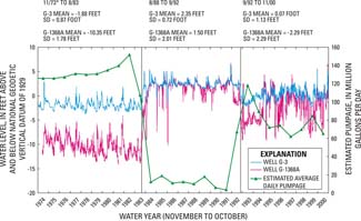Figure 5. Hydrograph showing variation in water levels at wells G-3 and G-1368A along with estimated average daily pumpage based on annual pumpage totals during water years 1974-2000. Link to larger version

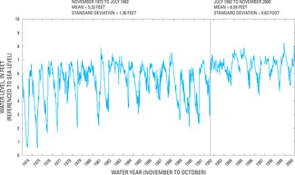Figure 6. Hydrograph showing variation in water level at well G-1502 during water years 1974-2000. Link to larger version

The comparison of aquifer water levels at wells G-3 and G-1368A (fig. 5) also depicts a slightly less apparent example of spatially distributed, temporal water-level variation. Before urbanization began in southern Florida, water levels in wells G-3 and G-1368A probably were nearly identical because these wells are only 1 mi apart. The differences in water-level behavior that exist now between wells G-3 and G-1368A are strongly influenced by variations in pumpage from the Hialeah-Miami Springs Well Field (fig. 5). Using this line of reasoning, if wells G-3 and G-1368A had historical water-level data from the last few centuries, a correlation analysis of the data for this entire period likely would yield a correlation coefficient that approaches 1.0 (representing excellent correlation because nearly all of the data being compared would be from the period prior to well-field installation. In this example, however, the result of the correlation analysis would probably not be very representative of current conditions. Considering the changes that have occurred in this area and that have affected water-level data from both wells, a long-term correlation analysis alone would not be an appropriate approach.

Next: Evaluating Correlation of Water-Level Data