Click on figures for larger images.

Figure 5. Port-side view of the National Oceanic and Atmospheric Administration Ship Thomas Jefferson at sea.

Figure 6. The National Oceanic and Atmospheric Administration Launch 1014 being deployed from the NOAA Ship Thomas Jefferson.

Figure 7. A Klein 5000 sidescan-sonar system hull-mounted to a National Oceanic and Atmospheric Administration launch.

Figure 8. The RESON Seabat 8101 hull-mounted in the keel cut out of National Oceanic and Atmospheric Administration Launch 1005.

Figure 9. The RESON Seabat 8125 hull-mounted in the keel cut out of National Oceanic and Atmospheric Administration Launch 1014.

Figure 10. Conductivity-temperature-depth (CTD) profiler.

Figure 11. A port-side view of the USGS research vessel Rafael that was used to collect Chirp and Boomer seismic-reflection profiles, bottom photography, and sediment samples in the vicinity of Edgartown Harbor, Massachusetts.

Figure 12. The locations of the tracklines (blue lines) along which the 5 Boomer high-resolution seismic-reflection profiles were collected during cruise 08034 of research vessel Rafael.

Figure 13. The locations of the tracklines (green lines) along which the 16 Chirp high-resolution seismic-reflection profiles were collected during the August 2008 cruise 08034 of the research vessel Rafael.

Figure 14. The small Seabed Observation and Sampling System (SEABOSS), a modified Van Veen grab equipped with still and video photographic systems, mounted on the aft starboard side of the research vessel Rafael.

Figure 15. Locations of stations at which bottom samples and photographs were taken during cruise 08012 of research vessel Rafael to verify acoustic data.

Figure 16. Correlation chart showing the relationships among phi sizes, millimeter diameters, size classifications (Wentworth, 1922), and American Society for Testing and Materials and Tyler sieve sizes.

Figure 17. Sediment-classification scheme from Shepard (1954), as modified by Schlee (1973).

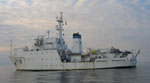
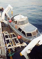
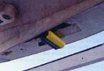
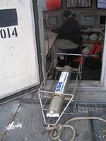
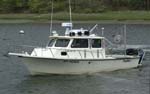
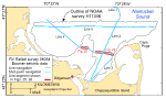
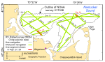
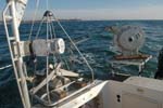
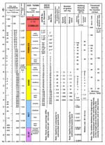
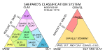
Sidescan Sonar and Bathymetry

Two 29-foot aluminum Jensen launches (1014 and 1005) deployed from the NOAA Ship Thomas Jefferson acquired sidescan-sonar and single-beam and multibeam bathymetric data from an area of sea floor of approximately 37.3 km² during 2004 (figs. 5, 6). The sidescan-sonar data were acquired with Klein 5000 sidescan-sonar systems hull-mounted to the launches (fig. 7). The systems were set to sweep 100 m to either side of the launch tracks. The systems emitted port and starboard 50°-wide beams tilted down 20° from horizontal and transmitted at 455 kHz. Daily confidence checks were made of the sidescan-sonar system by observing the outer ranges of the sonar images. The data were acquired in XTF (extended Triton data format), recorded digitally through an ISIS data-acquisition system, and processed by using CARIS SIPS (Sidescan Image Processing) software for quality control, and to produce a composite sidescan-sonar image at 2-m horizontal resolution. As part of this process, the sidescan-sonar data were demultiplexed and filtered to remove speckle noise and to correct for slant-range distortions. Image shine through to account for areas of overlap and auto-contrast adjustment were applied. Contrast enhancement based on the dynamic range of the data was applied to the mosaic, and it was then projected into UTM Zone 19 to produce an enhanced image.  Adobe Photoshop CS2 and ArcGIS 9.2 were used to refine the grayscale stretch and enhance the imagery.

The single-beam bathymetric data were collected with an Odom vertical-beam echosounder. The single-beam bathymetry data were supplemented by multibeam echosounder data that were collected with hull-mounted RESON SeaBat 240-kHz 8101 and 455-kHz 8125 shallow-water systems (figs. 8, 9). These systems measure two-way sound traveltime across a 150-degree swath and 120-degree swath, respectively. The SeaBat 8101 has 101 beams at a 1.5-degree beam spacing. The SeaBat 8125 has 240 beams with a cross-track beam width of 0.5 degrees at nadir. Original horizontal resolution of the multibeam bathymetric data was 0.5 m; vertical resolution of the multibeam data is about 0.5 percent of the water depth. Both bathymetric datasets were acquired in XTF (extended Triton data format), recorded digitally through an ISIS data acquisition system, and processed by NOAA, which used CARIS HIPS (Hydrographic Image Processing System) software to control quality, incorporate sound-velocity and tidal corrections, and produce a digital terrain model. Because of the areas of no data between ship tracks, the bathymetric data were regridded to 25 m at the USGS Woods Hole Coastal and Marine Science Center and interpolated to eliminate data gaps and to create continuous-coverage datasets. A more detailed description of the acquisition parameters and processing steps performed by NOAA and the USGS to create the datasets presented in this report are included in the metadata files. These files can be accessed through the Data Catalog section of this report.

Navigation was by TSS POS/MV 320 differential global-positioning-system (GPS)-assisted inertial navigation systems; Hypack MAX was used for acquisition-line navigation. Sound-velocity corrections were derived by using frequent SEACAT CTD (conductivity-temperature-depth) profiles (fig. 10). Typically, a CTD cast was conducted every four to six hours of multibeam acquisition. Tidal-zone corrections were calculated from data acquired at the Nantucket tidal gauge and a tertiary tide gauge installed for this project at Edgartown, Massachusetts.

Seismic Reflection, Sampling, and Photography

The bathymetric and sidescan-sonar data were verified with Boomer and Chirp high-resolution seismic-reflection data during August 2008 aboard the research vessel (RV) Rafael during cruise 08034 and with sediment samples and bottom photography during September 2008 aboard the RV Rafael during cruise 08012 (fig. 11). The Boomer seismic data were acquired digitally along five lines totaling approximately 27.6 km in length with a GeoAcoustics Boomer source, GeoAcoustics power supply, Benthos AQ4 single-channel streamer, and Chesapeake Systems SonarWiz acquisition software (fig. 12). The Boomer was fired at a rate of 0.5 seconds at a power output of 175 joules. The received signal was filtered between 100 and 3000 Hz with a GeoPulse receiver. The Boomer trace data recorded for 266 ms with a sample rate of 0.533 ms in standard SEG-Y format. The 3.5-kHz Chirp data were acquired digitally along 16 lines totaling approximately 56.1 km in length with a Knudsen Engineering Limited (KEL) Chirp 3200 shallow-water system and KEL Sounder Suite software (fig. 13). The Chirp trace data were recorded with a ping rate of 0.5 seconds for 66 ms with a sample rate of 0.048 ms in standard SEG-Y format.

The raw Boomer and Chirp SEG-Y data were read into Promax R2003 processing software. Heave-compensation data from the Teledyne TSS sensor (mounted on the transducer sidemount pole) were extracted from the SEG-Y headers and were used to apply a static shift to the trace data and to mute the water column. An automatic gain control (AGC) with a window length of 5 ms was applied. The processed data were written to a new SEG-Y file, and Seismic Unix was used to read the processed SEG-Y files and extract shot number, horizontal position, year, day, and time of day. Shot-point navigation data for both Boomer and Chirp datasets were converted to point and line shapefiles in ArcCatalog.

Surficial-sediment samples (collected 0-2 cm below the sediment-water interface) and bottom photographs were collected at 37 stations with a modified Van Veen grab sampler equipped with still- and video-camera systems (figs. 14, 15). The photographic data were used to appraise intrastation bottom variability, faunal communities, and sedimentary structures (indicative of geological and biological processes) and to observe boulder fields where samples could not be collected. A gallery of images collected as part of this project is provided in the Bottom Photography section; location information for the bottom photographs can be accessed through the Data Catalog section.

In the laboratory, the sediment samples were disaggregated and wet-sieved to separate the coarse and fine fractions. The fine fraction (diameters less than 62 microns) was analyzed by Coulter Counter, the coarse fraction was analyzed by sieving, and the data were corrected for salt content. Sediment descriptions are based on the nomenclature proposed by Wentworth (1922; fig. 16), the inclusive graphics statistical method of Folk (1974), and the size classifications proposed by Shepard (1954; fig. 17). A detailed discussion of the laboratory methods is given in Poppe and others (2005). Because biogenic carbonate shells commonly form in situ, they usually are not considered to be sedimentologically representative of the depositional environment. Therefore, gravel-sized bivalve shells and other biogenic carbonate debris were ignored. The grain-size-analysis data can be accessed through the Data Catalog section of this report and in the Sediments section.

To facilitate interpretations of the distributions of surficial sediment and sedimentary environments, these data were supplemented by sediment data from compilations of earlier studies (Poppe and others, 2003) and unpublished datasets from the National Geophysical Data Center. The interpretations of sea-floor features, surficial-sediment distributions, and sedimentary environments presented herein are based on data from the sediment-sampling and bottom-photography stations, on tonal changes in backscatter on the imagery, and on the bathymetry. For the purposes of this paper, bedforms are defined by morphology and amplitude. Sand waves are higher than 1 m; megaripples are 0.2 to 1 m high; ripples are less than 0.2 m high (Ashley, 1990). The bathymetric grids and imagery released in this report should not be used for navigation.