Figure 2. Illustration of the geophysical systems used to define the geologic framework. Sidescan-sonar, swath-bathymetric, and seismic-reflection systems were used to define the surficial sediment distribution, depth, and underlying geology. Sampling systems were used to collect direct samples of the river-bed sediment. Differential Global Positioning System (DGPS) was used to navigate the instrumentation. Click on figure for larger image.

Figure 3. U.S. Geological Survey R/V Rafael with 234-kHz SWATHplus transducers mounted on the bow. (Photograph by D. Foster, U.S. Geological Survey). Click on figure for larger image.

Figure 4. Map displaying the SWATHplus interferometric-sonar and Chirp subbottom profiler tracklines and sound-velocity profile locations: (A) in the northernmost St. Clair River area (Klein sidescan-sonar data also were collected along shore-parallel tracklines); (B) at Marysville, Mich.; and (C) at Port Lambton, Ontario. Tracklines are shown in red and sound-velocity profile locations are shown in yellow. 2005 orthophoto base from Michigan State University, Remote Sensing & GIS Research and Outreach Services, USDA–SA Aerial Photography Field Office. After Foster and Denny, 2009. Click on figure for larger image.

Figure 5. Map showing tracklines in the northernmost St. Clair River area. Tracklines are shown in red. 2005 orthophoto base from Michigan State University, Remote Sensing & GIS Research and Outreach Services, USDA–FSA Aerial Photography Field Office. After Foster and Denny, 2009.Click on figure for larger image.

Figure 6. Color-shaded relief images of the bathymetry collected by the USGS in the St. Clair River. All depths are relative to the International Great Lakes Datum, 1985. Hillshade parameters: azimuth is 45 degrees, altitude is 15 degrees, and vertical exaggeration is 2 times. (A) Northernmost St. Clair River area. Depths range from approximately 151 to 175 meters; (B) At Marysville, Mich., depths range from approximately 164 to 175 meters; (C) At Port Lambton, Ontario, depths range from approximately 159 to 174 meters. 2005 orthophoto base from Michigan State University, Remote Sensing & GIS Research and Outreach Services, USDA–FSA Aerial Photography Field Office. Click on figure for larger image.

Figure 7. Map showing the acoustic backscatter collected by the USGS from the St. Clair River. High acoustic backscatter is displayed as light tones in the imagery and low acoustic backscatter is displayed as dark tones in the imagery; (A) northernmost survey area within the St. Clair River; (B) at Marysville, Mich.; and (C) at Port Lambton, Ontario. 2005 orthophoto base from Michigan State University, Remote Sensing & GIS Research and Outreach Services, USDA–FSA Aerial Photography Field Office. Click on figure for larger image.

Figure 8. The U.S. Geological Survey Mini SEABOSS, shown (left) being deployed from the RV Rafael was used to collect sediment samples, and to take video, and digital photographs. The Mini SEABOSS components viewed from below (right) are: (A) forward video camera; (B) downward video camera; (C) video light; (D) digital still camera and housing; (E) strobe light; (F) parallel lasers for scale; (G) laser for ranging; (H) junction block; (I) Van Veen grab sampler; (J) multiconducting cable. (Photographs by D. Blackwood, U.S. Geological Survey.) Click on figure for larger image.

Figure 9. Map showing locations and tracklines of video drifts (red lines), locations of individual digital still photographs (green dots), and sediment-sampling locations (yellow dots) for data acquired with the Mini SEABOSS in the St. Clair River. The red dots show locations of selected observations of video along video transects from Krishnappan (2009). 2005 orthophoto base from Michigan State University, Remote Sensing & GIS Research and Outreach Services, USDA–FSA Aerial Photography Field Office. After, Foster and Denny, 2009. Click on figure for larger image.

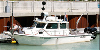
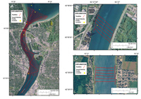
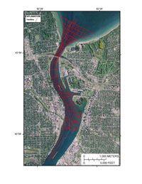
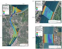
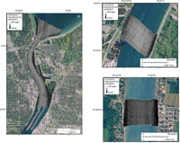
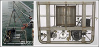
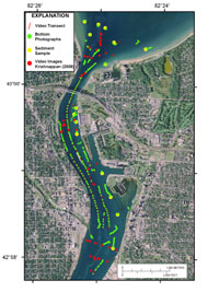
The following sections provide basic descriptions of shipboard acquisition and processing of the geophysical and sample data contained in this report. Detailed descriptions of acquisition parameters, processing steps, and accuracy assessments for each data type are provided in the geospatial metadata (see Data Catalog).

St. Clair River Field Program

Geophysical data, which were used to image the riverbed and subsurface morphology and sediments, were collected with Chirp and Boomer subbottom profilers, dual-frequency sidescan sonar, and a swath-bathymetric system (fig. 2). Video, photographs, and sediment samples of the riverbed were also collected using the USGS Mini SEABOSS (Blackwood and Parolski, 2001) to provide ground truth for the geophysical data. These systems were deployed from the R/V Rafael (fig. 3), a 7.6-m USGS research vessel operated by the Woods Hole Coastal and Marine Science Center (WHCMSC). Navigation data acquired during cruise operations were recorded by using HYPACK, Hydrographic Survey Software (HYPACK, Inc., 2010). Data were collected from May 29 to June 4, 2008, along tracklines spaced approximately 75 m apart parallel to the shore within a region from 2 km south of the Black River to 1 km north of the head of the St. Clair River in Lake Huron. Cross-channel survey lines were oriented at perpendicular or oblique angles to the shore-parallel tracklines (fig. 4a and fig. 5). Two site-specific surveys located to the south at Marysville, MI (fig. 4b), and Port Lambton, Ontario (fig. 4c), each covered approximately 500-m lengths of the river. These areas were surveyed to compare the geologic framework of the southern with that of the northern reaches of the St. Clair River. Sites were chosen based on ongoing studies as part of the IUGLS (Best and others, 2009; Yuzyk and Stakhiv, 2009).

Swath Bathymetry and Acoustic Backscatter

Swath-bathymetric and acoustic-backscatter data were acquired with a Systems Engineering and Assessment, Ltd., (SEA) SWATHplus interferometric sonar operating at a 234-kHz frequency (SEA, 2009). A total of 109 km of swath-bathymetric data was collected. The SWATHplus transducer was mounted at the bow of the R/V Rafael (fig. 2). A CODA Octopus F180 Attitude and Positioning system (Coda Octopus Group Inc., 2009) recorded ship motion (heave, pitch, roll, and yaw) and differential global positioning system (DGPS) corrected navigation. Additional navigation was recorded with a DGPS receiver positioned directly over the SWATHplus transducers. Horizontal and vertical offsets between navigation and attitude antennas and the SWATHplus transducer were recorded within the CODA Octopus F180 and SWATHplus configuration files, and the offsets were applied as the data were acquired. SWATHplus data-acquisition software was used to digitally record the bathymetric data at 4,096 samples per swath (ping). Bathymetric data were acquired over variable swath widths that ranged from 10 to 100 m, in water depths of about 1 to 25 m. Eight sound-velocity profiles were acquired during survey operations at roughly 4-hr intervals by using an Applied Microsystems SV Plus V2 Velocimeter (Applied Microsystems, 2009) (fig. 4). Variations in the speed of sound within the water column will affect the path of the acoustic ray as it travels from the transducer to the riverbed and back, introducing artifacts in the data. In order to minimize refraction artifacts, sound-velocity profiles were collected throughout the survey area in order to model the sound-velocity structure of the water column.

DGPS navigation was used to record the horizontal and vertical positions (x,y,z) of bathymetric soundings during data acquisition aboard the R/V Rafael. Real Time Kinematic GPS (RTK–GPS) corrections were applied to the navigation data during post-processing to provide sub-meter horizontal and vertical accuracies of the soundings. Fort Gratiot, MI, a Continuously Operating Reference Station (CORS) (National Geodetic Survey, 2009), was used as the reference station for the RTK-GPS corrections. A RTK–GPS base station was established at the tidal benchmark at the U.S. Coast Guard Base at Port Huron in order to determine the offset between the North American Vertical Datum of 1988 (NAVD 88) (vertical datum referenced at the CORS site) and the International Great Lakes Datum 1985 (IGLD 1985) referenced at the tidal benchmark. The following offsets were applied to the shipboard DGPS data during processing: the vertical offset between NAVD 88 and IGLD 85, the measured distance between the DGPS antenna and SWATHplus transducer, and the depth of the transducer below the water line. The resulting values were applied to the bathymetric soundings during processing to provide a measure of depth relative to IGLD 85.

Bathymetric data were processed by using SWATHplus (SEA, 2009) and Computer Aided Resource Information System (CARIS) (CARIS, 2009). During processing data were filtered to remove spurious soundings, rectified for ship motion, and corrected for speed-of-sound changes within the water column (SEA, 2009). RTK–GPS corrections were then applied to the soundings to provide improved vertical resolution and depth relative to IGLD 85 (CARIS, 2009). The processed data were used to generate 1-m- and 0.5-m resolution bathymetric grids (fig. 6).

Backscatter data were extracted from the raw SWATHplus data files and converted to USGS Xsonar/Showimage file format (Danforth, 1997) using SwathEd swath-bathymetric processing software (Hughes Clarke, 1998). Radiometric and geometric distortions in the backscatter data were corrected using Xsonar/Showimage following the methodology of Danforth (1997). A georeferenced acoustic backscatter mosaic was generated at a pixel resolution of 0.5 m and converted to a TIFF image (Hughes Clarke, 1998). A linear stretch, used to translate the observed digital-number range within the imagery to the full range of the data (a digital number range of 0–255 for an 8-bit grayscale image) was applied to enhance the dynamic range of these data (fig. 7).

A total of 59 km of sidescan-sonar backscatter data was collected with a Klein Associates, Inc., System 3000 dual-frequency sonar operating at 132- and 445-kHz (Klein Associates Inc., 2009). The Klein system was deployed off the port side of the R/V Rafael and towed less than 5 m astern. Horizontal and vertical offsets between the sonar towfish and the DGPS antenna were measured and recorded within SonarPro acquisition software in order to calculate towfish position (Triton Imaging, Inc., 2009). Data were collected at a 0.033-s sampling rate yielding a 100-m swath width. Data were logged and stored in eXtended Triton format (XTF) by using SonarPro (Triton Imaging, Inc., 2009).

The Klein sidescan-sonar data were processed following the methodology of Danforth and others (1991), Danforth (1997), and Paskevich (1996) to remove radiometric and geometric distortions in the raw data. Processed sonar data were mosaicked digitally following the procedures described in Paskevich (1996) using PCI Geomatics OrthoEngine (PCI Geomatics, 2009). The georeferenced mosaic was projected in Universal Transverse Mercator (UTM) 17N coordinates, referenced to the WGS84 datum at a 0.5-m pixel resolution. The mosaic was saved in TIFF format, and a linear stretch was applied.

The SWATHplus and Klein backscatter mosaics were compared to identify the device that provided the highest quality of imagery. The SWATHplus mosaic contained less acoustic noise than the Klein mosaic, most likely due to the mount position of the SWATHplus sonar. The sonar head was mounted on the bow of the R/V Rafael, far enough from the propellers to prevent noise from distorting the sonar signals and the resulting images. The Klein sonar system, however, was towed off the stern of the vessel and was in close proximity to the propellers. As a result, the SWATHplus mosaic was used for feature identification and interpretation due to the higher quality of the mosaic. The Klein mosaic was not used and is not included in this report.

Subbottom Profiling

A total of 80 km of sub-bottom data was collected by using a dual-frequency (3.5- and 200-kHz) Knudsen Engineering Limited (KEL) Chirp 3200 system (Knudsen Engineering Limited, 2009) (fig. 4 ). The single-beam water depths from the 200-kHz channel were logged together with navigation in ASCII format. Chirp subbottom data with a peak frequency of 3.5 kHz provided a vertical resolution of approximately 30 cm. The Chirp system was fired at a rate of 0.25 or 0.5 s. The trace length was set to 67 ms. The data were recorded in Society of Exploration Geophysicists Y (SEG-Y) format (Barry and others, 1975) with DGPS navigation logged to the SEG-Y file trace headers.

A total of 58.5 km of subbottom data was collected by using a subbottom profiling system (fig. 5 ). Compared to the , the system provided a higher energy source operating at 175 joules and provided deeper penetration of the underlying stratigraphy. With a peak frequency of about 1,800 Hz, the vertical resolution was approximately 1 m. The layback distance from the DGPS antenna to the source and receiver was estimated and applied to the position data during acquisition. The was fired at 0.5 s, and each trace was recorded with 200 ms of data. The data were acquired in SEG-Y format by using SonarWiz.MAP +SBP software (Chesapeake Technology Inc., 2009). Shot-point navigation recorded DGPS location in the SEG-Y file trace headers.

Subbottom data were processed by using SIOSEIS (2009) and were loaded into SeisVision (Halliburton, 2009) seismic-interpretation software. The major unconformities were interpreted and digitized. Isochron data were exported and subsequently imported into EarthVision surface-modeling software (Dynamic Graphics, Inc., 2009). The data points were gridded at a 20 by 20-m cell size. Isochron values were converted to thickness in meters by using a constant sediment velocity of 1,650 m/s. This acoustic velocity correlated well with the depth to bedrock indicated by the geologic cross sections near the railway tunnels. We used a 5-m grid derived from our swath-bathymetric data and isopach grids to calculate the elevation (IGLD 85) surfaces.

Video and Photography

Video and photographs of the riverbed were collected at 37 stations by using the USGS Mini SEABOSS (U.S. Geological Survey, 2008; fig. 8; fig. 9). Mini SEABOSS stations were selected based on preliminary acoustic-backscatter mosaics, with the objective of characterizing broad areas of different backscatter intensity. With the Mini SEABOSS deployed, the research vessel was allowed to drift, with occasional power from the vessel applied to control drift direction. Continuous video was collected over a total of 11.5 km of lake and riverbed. Video drift position was extracted from the recorded HYPACK navigation files by using the start and end times of the drift. For some portions of the drift, there was no navigation, so the position was derived from the time and position stamp in the video at 30-s intervals. The full-resolution raw video files were archived to DVD-R and were then reduced to 640–to–480 pixels and converted to MPEG–4 format. A total of 449 photographs were obtained from a digital still camera at user-selected locations along the drifts. A Python script was used to merge drift navigation with digital photographs using time of day to synchronize the two data sources.

Sediment Samples

Samples of the surficial sediment were collected at 15 stations (fig. 9) using a Van Veen sampler configured on the Mini SEABOSS, typically at the end of a drift. The upper 2 cm of sediment was scraped from the surface of the sample for texture analysis. Sediment samples were collected at locations with relatively fine-grained sediment (sand or mud). Samples were not collected in gravel or cobble areas where gravel prevented full closure of the sampler and resulted in a washed-out sample.

A total of 13 bottom samples was submitted for grain-size analysis. Two partially recovered, washed-out samples were not submitted. Grain-size analysis was performed at the USGS Sediment Laboratory at WHCMSC by using methods described by Poppe and others (2005).