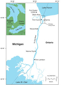USGS Home
Contact USGS
Search USGS

Geophysical Data Collected from the St. Clair River between Michigan and Ontario, Canada (2008-016-FA)

List of Figures

Title Page Contents List of Figures Conversion Factors Abstract Introduction Data Acquisition and Processing Data Catalog Acknowledgments References Cited

Figure 1. Map showing the St. Clair River. The primary study area lies in the northern reaches of the river, with two additional study sites offshore from Marysville, Mich., and Port Lambton, Ontario. Base map generated from data supplied by ESRI, ArcGIS 9.2. After Foster and Denny, 2009. Click on figure for larger image. Figure 2. Illustration of the geophysical systems used to define the geologic framework. Sidescan-sonar, swath-bathymetric, and seismic-reflection systems were used to define the surficial sediment distribution, depth, and underlying geology. Sampling systems were used to collect direct samples of the river-bed sediment. Differential Global Positioning System (DGPS) was used to navigate the instrumentation. Click on figure for larger image. 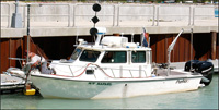Figure 3. U.S. Geological Survey R/V Rafael with 234-kHz SWATHplus transducers mounted on the bow. (Photograph by D. Foster, U.S. Geological Survey).Click on figure for larger image. 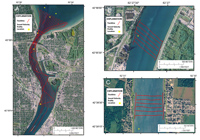Figure 4. Map displaying the SWATHplus interferometric-sonar and Chirp subbottom profiler tracklines and sound-velocity profile locations: (A) in the northernmost St. Clair River area (Klein sidescan-sonar data also were collected along shore-parallel tracklines); (B) at Marysville, Mich.; and (C) at Port Lambton, Ontario. Tracklines are shown in red and sound-velocity profile locations are shown in yellow. 2005 orthophoto base from Michigan State University, Remote Sensing & GIS Research and Outreach Services, USDA–FSA Aerial Photography Field Office. After Foster and Denny, 2009. Click on figure for larger image. 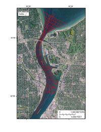Figure 5. Map showing Boomer subbottom tracklines in the northernmost St. Clair River area. Tracklines are shown in red. 2005 orthophoto base from Michigan State University, Remote Sensing & GIS Research and Outreach Services, USDA–FSA Aerial Photography Field Office. After Foster and Denny, 2009. Click on figure for larger image. 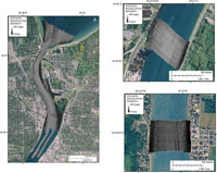Figure 6. Color-shaded relief images of the bathymetry collected by the USGS in the St. Clair River. All depths are relative to the International Great Lakes Datum, 1985. Hillshade parameters: azimuth is 45 degrees, altitude is 15 degrees, and vertical exaggeration is 2 times. (A) Northernmost St. Clair River area. Depths range from approximately 151 to 175 meters. (B) At Marysville, MI, depths range from approximately 164 to 175 meters. (C) At Port Lambton, Ontario, depths range from approximately 159 to 174 meters. 2005 orthophoto base from Michigan State University, Remote Sensing & GIS Research and Outreach Services, USDA-FSA Aerial Photography Field Office. Click on figure for larger image. 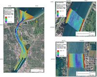Figure 7. Map showing the acoustic backscatter collected by the USGS from the St. Clair River. High acoustic backscatter is displayed as light tones in the imagery, and low acoustic backscatter is displayed as dark tones in the imagery. (A) Northernmost survey area in the St. Clair River; (B) at Marysville, Mich.; and (C) at Port Lambton, Ontario. 2005 orthophoto base from Michigan State University, Remote Sensing & GIS Research and Outreach Services, USDA–FSA Aerial Photography Field Office. Click on figure for larger image. 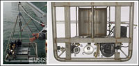Figure 8. The U.S. Geological Survey Mini SEABOSS, shown (left) being deployed from the RV Rafael was used to collect sediment samples, and to take video and digital photographs. The Mini SEABOSS components viewed from below (right) are: (A) forward video camera; (B) downward video camera; (C) video light; (D) digital still camera and housing; (E) strobe light; (F) parallel lasers for scale; (G) laser for ranging; (H) junction block; (I) Van Veen grab sampler; (J) multiconducting cable. (Photographs by D. Blackwood, U.S. Geological Survey.) Click on figure for larger image. 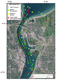Figure 9. Map showing locations and tracklines of video drifts (red lines), locations of individual digital still photographs (green dots), and sediment-sampling locations (yellow dots) for data acquired with the Mini SEABOSS in the St. Clair River. The red dots show locations of selected observations of video along video transects from Krishnappan (2009). 2005 orthophoto base from Michigan State University, Remote Sensing & GIS Research and Outreach Services, USDA&ndashFSA Aerial Photography Field Office. After Foster and Denny, 2009. Click on figure for larger image.