USGS OFR 2012-1178: Profile Measurements and Data From the 2011 Optics, Acoustics, and Stress In Situ (OASIS) Project at the Martha's Vineyard Coastal Observatory, Appendix A

Appendix 1. Arm Geometry

Click on figure for larger image

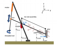Figure 9. Schematic diagram of the geometry and key components of a profiling arm. Refer to the Abbreviations and Symbols section. See the Instrumentation section for a complete description of these instruments.

This appendix describes the location of instruments on the profiling arm and methods for calculating the elevation of the instruments above the seafloor as the arm moved. Arm motion was monitored by a pair of two-axis tilt meters (SBG Systems IG-20 model A2P1-B two-axis inclinometer and three-axis accelerometer). One IG-20 was attached to the top of the arm 0.35 meter (m) outboard of the pivot point, and its readings were transmitted at 4 hertz (Hz) by the Modtronix Engineering SBC68EC single-board computer to the Moxa main control computer. The second IG-20 was mounted on the instrument package at the end of the arm, and its readings were recorded at 50 Hz by the Moxa. The pitch and roll axes of the arm IG-20 were aligned parallel to the arm (y-axis) and perpendicular (horizontally, x-axis) to the arm. Roll angles were very small (less than 2 degree (°) angle), and the average roll was 0.4°, so only pitch (referred to here as arm angle (α)) was needed in elevation calculations. Thus, the calculations discussed here are a two-dimensional (2D) representation of the geometry.

Table 1-1. Location of sensors on the profiling arm.

[Distances are in meters and are measured from the identified points. See the Instrumentation section for a complete description of these instruments. See also Abbreviations and Symbols]

Instrument	x_a	r_a	z_a	y_p	z_p
Location of sensors on the profiling arm. Distances in meters.
IG-20 (tilt)	0	0.35	0.03	0	0
ADV	0	1.76	0	0.09	-0.27
YSI CTD	-0.10	1.76	0	0.09	-0.20
Paros	0.115	1.76	0	0	-0.04
OBS	0.075	1.76	0	0.08	-0.185
IG-20 (arm accel)	0	1.76	0	0	-0.21
ABSS	0.135	1.76	0	0	-0.25
Transmissometer	0	1.56	0.105	0	0
LISST-HOLO	-0.095	1.53	-0.105	0	0
LISST-100X	-0.065	1.54	-0.11	0	0
BB2F	-0.21	1.54	-0.11	0	0
Intake	0	1.7	-0.055	0	0

The locations of sensors on the profiling arm are listed above in terms of horizontal distance to the right (positive) or left (negative) from the center of the arm (x_a), horizontal distance from the pivot along the arm axis (radial distance out the arm, r_a), vertical distance above the arm (z_a; when the arm is level α =0°). For those sensors on the articulated instrument package at the end of the arm, additional dimensions y_p and z_p describe their location relative to the end of the arm in the horizontal (along axis of the arm) and vertical directions, respectively.

The geometry is illustrated in fig. 9. The vertical angle (α') between the arm and the sensor location depended on the radial distance out the arm (r_a) and vertical offset from the arm (z_a):

α' = tan^-1(z_a / r_a)

(1-1)

The adjusted radial distance from the pivot (r') was:

r' = r_a(cos(α'))

(1-2)

Horizontal distance y from the pivot and vertical distance z from the seafloor were calculated as:

y = r'(cos(α + α')) + y_p and

(1-3)

z = h_pivot + r'(sin(α + α')) + z_p

(1-4)

where h_pivot is the elevation of the arm pivot above the seafloor.

These equations were used for instruments mounted along the arm and for instruments on the articulated package at the end of the arm. For instruments mounted along the arm, horizontal and vertical offsets y_p and z_p were zero. For instruments on the articulated package at the end of the arm, y_p and z_p were added to the position of the end of the arm calculated with z_a = 0 and r = r' = length of the arm (1.76 m).

Elevation h_pivot was measured on the dock (1.335 m) but changed during the deployment as the feet of the tripod settled into the seafloor. We used the pulse-coherent acoustic doppler profiler (PCADP) data to determine the elevation of the PCADP transducer (h_PCADP) every 2 hours during the deployment. These elevations were determined by calculating the burst-mean of the apparent range of the burst to the seafloor reported by each of the three PCADP beams, correcting for beam geometry and burst-median of pitch and roll of the burst, and calculating the vertical distance to the intersection of the plane formed by the three estimates of seafloor location. The time-varying estimate of the pivot elevation over the deployment was calculated as h_pivot = h_PCADP + 0.3 m, where 0.3 m was the (constant) elevation difference between the pivot and the PCADP transducer.