U.S. Geological Survey Open-File Report 2012-1178
Profile Measurements and Data From the 2011 Optics, Acoustics, and Stress In Situ (OASIS) Project at the Martha's Vineyard Coastal Observatory
| Click on figures for larger images |
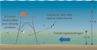 |
| Figure 2. Schematic illustration of profiling tripod with instruments on cantilever arm for profiling particle distributions in the bottom boundary layer. Refer to the Abbreviations and Symbols section. |
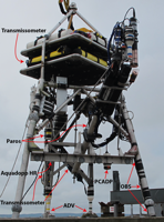 |
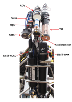
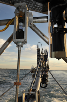
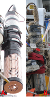
| Figure 3. Front view of the tripod with the profiling arm; frame-mounted instruments are labeled. Profiling arm is in the up position. See the Instrumentation section for a complete description of these instruments. |
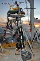 |
| Figure 6. Rear view of tripod with profiling arm; frame-mounted instruments are labelled. See the Instrumentation section for a complete description of these instruments. |
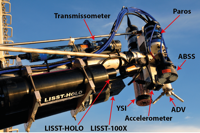 |
| Figure 7. Side view of profiling arm; instruments are labeled. See the Instrumentation section for a complete description of these instruments. |
 |
| Figure 8. Bottom view of profiling arm; instruments are labeled. See the Instrumentation section for a complete description of these instruments. |
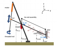 |
| Figure 9. Schematic diagram of the geometry and key components of a profiling arm. Refer to the Abbreviations and Symbols section. See the Instrumentation section for a complete description of these instruments. |
 |
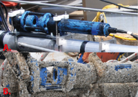
| Figure 10. Photograph of Technadyne rotary actuator, mount, and upper portion of drive screw. |
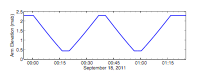 |
| Figure 11. Graph showing an example arm elevation time series for one profile cycle. Refer to the Abbreviations and Symbols section. |
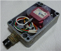 |
| Figure 12. Photograph of an SBG IG-20 two-axis inclinometer and three-axis accelerometer glued in the waterproof housing (lid removed). |
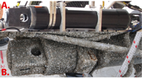 |
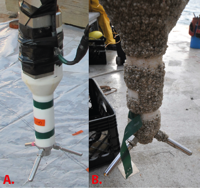
| Figure 13. Photograph of the Sequoia Scientific LISST-100X laser particle sizer on profiling arm A, before deployment and B, after recovery. |
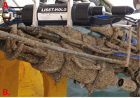 |
| Figure 14. Photograph of the Sequoia Scientific LISST-HOLO submersible digital holographic particle imaging system on profiling arm A, before deployment and B, after recovery. |
 |
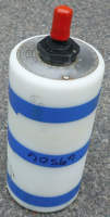
| Figure 15. Photograph of the YSI 6600 multiparameter sonde on profiling arm A, before deployment and B, after recovery. |
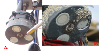 |
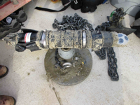
| Figure 16. Photograph of the Aquatec Aquascat acoustic backscatter system on profiling arm A, before deployment and B, after recovery. |
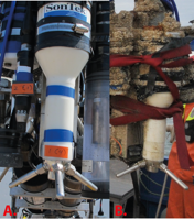 |
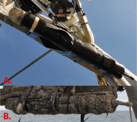
| Figure 17. Photograph of the SonTek ADV on profiling arm A, before deployment and B, after recovery. |
 |
| Figure 18. Photograph of the Paroscientific, (Paros) Digiquartz pressure sensor. |
 |
| Figure 19. Photograph of the D&A Instrument Company optical backscatter sensor (OBS) on the profiling arm before deployment. |
 |
| Figure 20. Photograph of Seatech 5-centimeter transmissometer on the profiling arm A, before deployment and B, after recovery. |
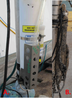 |
| Figure 21. Photograph of the Sea-Bird SEACAT mounted on a tripod leg 0.4 meters above the bottom A, before deployment and B, after recovery. |
 |
| Figure 22. Photograph of the Nortek Aquadopp HR velocity profiler mounted on the tripod crossbeam 1.08 meters above the bottom A, before deployment and B, after recovery. |
 |
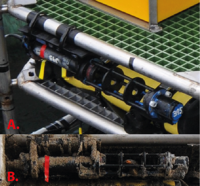
| Figure 23. Photograph of the SonTek PCADP mounted on the tripod crossbeam 1.03 meters above the bottom A, before deployment and B, after recovery. |
 |
| Figure 24. Photograph of the Seatech 25-centimeter transmissometer logged with the red PCADP and mounted on the tripod frame 2.75 meters above the bottom A, before deployment and B, after recovery. |
 |
| Figure 25. Photograph of the SonTek ADV (9105) mounted on the tripod frame 0.42 meter above the bottom A, before deployment and B, after recovery. |
 |
| Figure 26. Photograph of the SonTek ADV (9106) mounted on the tripod frame 0.42 meter above the bottom A, before deployment and B, after recovery. |
 |
| Figure 27. Photograph of the Nortek Aquadopp (9111) profiler mounted on a monopod 0.16 meter above the bottom after recovery. |
|
The profiling arm was attached to the existing "flowbee" tripod (figs. 3, 6, 7, and 8), originally built to support instruments for measuring waves, currents, and suspended sediments in shallow environments. The flowbee tripod was used previously off Cape Hatteras, North Carolina in 2009 and at the MVCO in summer 2005 and (with a modified immobile arm) in summer 2007. The flowbee tripod is constructed of stainless steel and is about 3.5 meters (m) tall, with feet about 1.9 m apart. The legs are stainless steel pipes with an outside diameter of 7.6 centimeters (cm). The feet are cylindrical lead weights 41 cm in diameter and 16.5 cm thick; they weigh 136 kilograms (kg). Two decks are located on the upper tripod to support instruments and battery cases; the bottom of the lower deck is approximately 2.6 m above the seafloor. The recovery package normally mounted on the top of the tripod was not used during this OASIS experiment because the recovery line was attached by divers.The profiling arm was designed to move an instrument package up and down between the seafloor and an elevation of about 2 meters above the bottom (mab). The design criteria for the arm were based on the scientific objectives of the OASIS program, as follows:
Arm DesignThe design of the profiling arm was based on a cantilever arm, with a fulcrum (pivot) on a crossbar of the tripod (figs. 2 and 9). The longer end of the arm extended 1.98 m beyond the tripod and supported the instruments, and the shorter lever end extended 0.71 m into the interior of the tripod. A long threaded stainless-steel rod passed through a gimbaled brass nut on the lever end. This screw was turned by an electric motor mounted high on the interior of the tripod; as the lever end was raised, the instrument end was lowered, and vice versa. The final design of the profiling arm incorporated minor improvements, such as universal mounts for the motor and brass nut, and thrust bearings to protect the motor from axial loads transferred by the screw. Details of the arm geometry are described in appendix 1.
Arm Interface and ControlThe interface between the Moxa main control computer and the Technadyne Model 20 arm actuator was a Modtronix Engineering SBC68EC single-board computer and custom daughterboard to limit power draw. Communication between the Moxa, the Modtronix arm controller, other components, and shoreside computers was via Ethernet. A detailed description of arm interface and control hardware and software is included appendix 2. Software used in the project for arm control and data logging is discussed in appendix 3. Arm Movement and Sampling ScheduleFour profiles (down, up, down, up) were made every 2 hours (hr) beginning on even hours (fig. 11), except when power to the MVCO node was turned off for maintenance. Each profile took about 16 min, with the end of the arm moving at a somewhat variable rate of approximately 2.2 millimeters per second. Normal profiles started with the arm up at an angle of 37 degrees (°; relative to horizontal) with the motor stopped. At the top of the even hour, a sequence of commands to supply power to the motor and begin arm movement was issued. Starting about 5 seconds (s) after the hour, motor speed was increased gradually over a period of about 20 s until the arm was rotating at a constant rate, causing the arm to move downward for about 16 min. Computers monitored the arm angle, and when it reached a predetermined value (initially, -27°; later reduced to -25.5°, then -24°), the motor was stopped, leaving the arm in the down position, where it remained until 20 min after the hour. At 20 min after the hour, the motor ramped up to a constant rotation rate in the opposite direction, moving the arm upward for about 16 min until it reached the up-position angle (37°). At 40 min past the hour, the sequence was repeated and the arm completed another pair of profiles.
Arm InstrumentsWe describe in this section the instruments that produced data from the profiling arm. For each instrument, we introduce an abbreviated name in parentheses (for example, ADV) for later reference. Numbers in parentheses in the section titles (for example, 9104) are the USGS mooring identification numbers, which link the instrument to data files in USGS archives. The mooring identification numbers are associated with data loggers, so all sensors with output recorded by a single logger (for example, a SonTek Hydra system) are associated with the same mooring identification number. Some instruments are described also by the colors used to mark their cables and sensors (for example, blue ADV), which helps match instruments and data with photographs documenting their location and condition. Logger and ControllersThe primary logger and controller for the profiling arm was the Moxa Linux computer. This computer issued instructions to the Modtronix arm controller and logged data sent by the Modtronix and several arm instruments. ModtronixThe Modtronix SBC68EC (http://www.modtronix.com/product_info.php?products_id=196) controlled the arm motor, monitored motor status and arm angle, and reported these data over the internal network in a user datagram protocol (UDP) datagram about 4 times per second. The contents of the datagrams were unpacked by the Moxa as they were received and written to an American Standard Code for Information Interchange (ASCII) data file on the Moxa. This file was retrieved by the shoreside computer after each set of profiles. The datagrams included a time stamp with the system time, data (time since reset, roll and pitch angles, three axes of acceleration, and two onboard temperatures) sent to the Modtronix from the tilt meter on the arm, and data (status of motor power, motor current draw, motor rotation rate, control voltage sent to the motor, and status of the software circuit breaker) acquired by the Modtronix from the motor-controller circuit board. MoxaThe Moxa UC8418 computer (http://www.moxa.com/product/UC-8418.htm) logged data from several instruments on the arm. These included all data from the SBG Systems IG-20 two-axis inclinometer and three-axis accelerometer at the end of the arm, all data from the YSI 6600 multiparameter sonde on the end of the arm, all data from the SonTek pulse-coherent acoustic doppler profiler (PCADP) mounted on the crossbar of the tripod, and header information from the SonTek acoustic doppler velocimeter (ADV) on the end of the arm. Following each 2-hour profiling period, the data files were written to a directory on the solid-state disk mounted on the Moxa as /var/sda/data and also copied back to the shoreside computer.
Arm accelerometer (IG-20)Two IG-20 tilt meter and accelerometer units (http://www.sbg-systems.com/products/ig-20) were mounted on the arm, one to monitor the angle of the arm and the other to monitor the motion of the instrument package at the end of the arm (figs 7 and 8). The IG-20s were compact (36 × 49 × 22 millimeters (mm)) and lightweight (38 grams (g)) and required small amounts of power (less than 150 milliwatts (mW)) (fig. 12). According to the manufacturer, they could measure pitch and roll over a range of ±80° and ±180° (respectively) with a static accuracy of ±0.2° and a resolution of less than 0.05°. The accelerometers measured over a range of ±2 g, with nonlinearity of less than 0.2 percent of the full scale, bias stability of ±0.002 g, and alignment error of less than 0.1 over a bandwidth of 0.1 to 100 hertz (Hz).
Sequoia Scientific LISST-100X (LISST-100X) - 9109The Sequoia Scientific Laser In Situ Scattering and Transmissometry 100X (LISST-100X; http://www.sequoiasci.com/products/susp_LISST_100.aspx) laser particle sizer (fig. 13) uses a collimated laser and an annular ring detector to measure forward scattering by particles along the optical path. The forward scattering data are mathematically inverted to provide an estimate of the volume concentration (in microliters per liter, µL/L) of particles in 32 log-spaced-size classes. This system can resolve particles ranging from 2.5 to 500 microns (micrometers, µm) in diameter. In addition to particle size distribution, the LISST-100X measures the percentage of transmission along the optical path, temperature, and pressure.
Sequoia Scientific LISST-HOLO (LISST-HOLO) - 91010The LISST-HOLO (http://www.sequoiasci.com/products/fam_LISST_HOLO.cmsx) in situ in-line holographic camera (fig. 14) illuminates a 5-cm optical path with a red (658-nanometer (nm)-wavelength) collimated laser. Particles in the water scatter the laser light along the optical path. A charge-coupled device (CCD) opposite the laser captures particle silhouettes and the interference pattern created by the interaction of scattered and unscattered light. Subsequent processing uses the interference patterns to identify and digitally focus on particles in narrow slices along the length of the optical path. Image analysis algorithms can be used to characterize the size and shape of the imaged particles.
YSI 6600 Multiparameter Sonde (YSI) - 91011The YSI model 6600 multiparameter sonde (http://www.ysi.com/productsdetail.php?6600V2-1) is a water-quality sensor that uses interchangeable probes to measure a variety of parameters (fig. 15). For this study, the sonde was equipped with conductivity, temperature, pressure, dissolved-oxygen, and turbidity probes.
Aquatec Acoustic Backscatter System (ABSS) - 91012The Aquatec acoustic backscatter system (ABSS; http://www.aquatecgroup.com/index.php/products/aquascat) emits pulses of high-frequency sound from up to four transducers at a variety of frequencies (fig. 16). The pulses are scattered by suspended material in the water column. The ABSS measures the scattered sound returned from particles in the water column and produces vertical profiles of acoustic backscatter intensity (a proxy for suspended sediment concentration). This system uses three transducers of differing frequency (1 megahertz (MHz), 2.5 MHz, and 4 MHz) and measures profiles of backscatter intensity in very small bins (mm to cm). In general, lower frequency sound is more responsive to larger particles so comparing the response of multiple frequencies can provide information on the size of particles in suspension.
SonTek Acoustic Doppler Velocimeter-Ocean and Hydra logger (Blue ADV) - 91013The SonTek Acoustic Doppler Velocimeter-Ocean (blue ADV) was connected to a Hydra system, an electronics package in an underwater housing that controls instruments, provides power, and records data. The Hydra system accommodates the 5-MHz ADVOcean probe (fig. 17) as well as numerous user-configurable external sensors (for example, pressure sensors or optical turbidity sensors). For this study, several instruments were associated with a color, blue, for example, used on cases and cables to distinguish all sensors logged by a particular Hydra logger. The Hydra logger and associated sensors used on the arm array were color-coded blue.
SonTek ADVOcean Acoustic Doppler Velocimeter (ADV)The 5-MHz SonTek ADVOcean (ADV; http://www.sontek.com/advocean-hydra.php) makes three-component vector measurements of water flow using doppler principles and records them with synchronous measurements from an array of complementary external sensors.
Paroscientific, Digiquartz Pressure Sensors (Paros)The Paroscientific, (Paros) Digiquartz pressure sensor (http://www.paroscientific.com/Depthsensors.htm) measures pressure using a quartz crystal resonator. The frequency of oscillation of this resonator varies with pressure induced stress. The output pressure is compensated for temperature by using the signal from temperature-sensitive crystals within the instrument.
D&A Instrument Company Optical Backscatter Sensor (OBS)The D&A Instrument Company OBS-3 sensor (fig. 19) measures optical backscatter, a proxy for suspended solids concentration (SSC), in the water column. The sensor emits a beam of infrared light that is scattered by suspended solids. Optical backscatter sensors can be calibrated in the laboratory to provide data in units of turbidity or by using suspended solid samples collected in situ to provide information about suspended solid concentrations. Prior to deployment, all OBS sensors were intercalibrated in the laboratory using a Formazin calibration standard and a multistep (0 nephelometric turbidity units (NTU), 5 NTU, 15 NTU, 30 NTU, 50 NTU, 100 NTU, 300 NTU, and 500 NTU) calibration procedure.
Sea Tech TransmissometerThe Sea Tech transmissometer (fig. 20) measures the transmission of red collimated light (660-nm wavelength) through the water. The percent transmission of light and the length of the optical path (5 cm or 25 cm) can be used to calculate an attenuation coefficient. Transmission and attenuation are often used as proxies for SSC in the water column.
University of Maine ECO BB2F Spectral Backscattering Meter and CDOM Fluorometer (BB2F)The WETLabs ECO BB2F (http://www.wetlabs.com/products/ebb/bbvsfindex.htm) provided by the University of Maine is a combination scattering meter and fluorometer that measures backscattered light (at an angle of 117°) at two wavelengths (532 nm and 650 nm) and colored dissolved organic matter (CDOM) fluorescence (excited at 380 nm and emitted at 460 nm). The BB2F was mounted near the end of the profiling arm. Data were recorded at 2 Hz. Computation of the particulate backscattering coefficient from single measurements in the back direction was done following Boss and others (2004). The CDOM fluorometer channel did not work during the deployment (no change in very noisy data) and those data are not included in this report. The BB2F was not equipped with automatic wipers and was too delicate to be cleaned by divers. University of Maine AC-9 Spectral Absorption and Beam Attenuation Meter (AC-9)The WetLabs AC-9 spectral absorption and beam attenuation meter (http://www.wetlabs.com/products/ac/acall.htm) provided by the University of Maine measures attenuation and absorption of light at nine wavelengths (412 nm, 440 nm, 490 nm, 510 nm, 532 nm, 555 nm, 650 nm, 676 nm, and 715 nm). Water sampled by the AC-9 was pumped from an intake mounted near the end of the arm. A valve allowed the flow to be routed directly to the AC-9 or through a filter and then to the AC-9. The filter removed particles larger than 0.2 µm from the sample, which allowed for calculations of particulate absorption and attenuation that were calibration independent (see Boss and others, 2007; Slade and others, 2011). Data from the sensor was recorded at 6 Hz. Chlorophyll-a concentration (Chl) was computed from the absorption line height at 676 nm (Boss and others, 2007). Mean size tendency or power-law slope (γ) of the power-spectral density was computed from attenuation spectra (Boss and others, 2001).
Tripod InstrumentsWe describe in this section the instruments that were mounted in fixed positions on the main frame of the tripod. For each instrument, we introduce an abbreviated name in parentheses, (for example, ADCP) for later reference. The numbers in parentheses in the section titles (for example, 9101) are the USGS mooring identification numbers, which link the instrument to data files in USGS archives. In addition, some instruments are described by the colors used to mark their cables and sensors (for example, green ADV), which helps match instruments and data with photographs documenting their location and condition. Teledyne RD Instruments Acoustic Doppler Current Profiler (ADCP) - 9101The 1,200-kilohertz (kHz) Teledyne RD Intruments (RDI) ADCP (abbreviated to ADCP here; http://www.rdinstruments.com/sen.aspx) measures the speed and direction of water flow using doppler principles. Acoustic pulses are transmitted by the ADCP transducer assembly along two pairs of orthogonal beams (four beams total). Scatterers in the water column, such as small sediment particles and plankton traveling with the water flow, reflect the acoustic pulses. The ADCP transducer assembly receives the reflected pulses and, using the doppler effect and basic trigonometry, converts the pulses into eastward, northward, and vertical components of water flow. When installed with waves acquisition firmware, RDI ADCPs record three different types of time series from which wave properties may be computed: pressure, range to surface along each orthogonal beam (that is, water level), and orbital velocities of the surface waves taken from three bins nearest the surface in each of the four beams. It is possible to estimate nondirectional wave energy spectra, and thus wave height and period, from any of the three time series, but the orbital velocity time series are required for definition of the directional distribution of the wave energy.
Sea-Bird Electronics 16plus V2 SEACAT (SEACAT) - 9102 and 9107The Sea-Bird Electronics 16plus V2 SEACAT recorder (SEACAT; http://www.seabird.com/products/spec_sheets/16plusdata.htm) is a conductivity and temperature (CT) sensor. Salinity can be determined from the conductivity and temperature record. The SEACATs are equipped with pumps to flush the sensor ducts and reduce salinity spiking and powered by internal batteries; data are recorded internally on flash random-access memory (RAM), allowing the instrument to operate autonomously.
Nortek Aquadopp High-Resolution Acoustic Profiler (Aquadopp HR) - 9103The Nortek AS Aquadopp 1-MHz high-resolution acoustic profiler (Aquadopp HR; http://nortekusa.com/usa/products/current-profilers/aquadopp-hr-profiler) uses acoustic doppler technology to measure 3D water flow velocity profiles. The Aquadopp HR is an upgraded version of the standard Nortek Aquadopp profiler. The Aquadopp HR uses a pulse-coherent processing technique to measure three components of velocity in small depth bins (2-30 cm) over a limited part (less than 6 m) of the water column.
SonTek Pulse Coherent Acoustic Doppler Profiler (Red PCADP) - 9104The 1.5-MHz SonTek PCADP has three acoustic beams and uses acoustic doppler technology to measure profiles of all three components of water velocity. Pulse-to-pulse processing allows this unit to measure velocity in small depth (about 6 cm) bins over a limited part (less than 5 m) of the water column.
SonTek Hydra ADVs (Green ADV 9105 and Yellow ADV 9106)A pair of SonTek ADVOcean acoustic doppler velocimeters (ADV) and Hydra systems, each with an external Paros pressure sensor, a D&A OBS, and a 5-cm Seatech transmissometer, were mounted on the tripod frame (individual sensors are described in previous sections). The green ADV (9105; fig. 25) had an ADVOcean probe mounted 0.42 mab, a Paros pressure sensor mounted 1.53 mab, a 5-cm Sea Tech transmissometer mounted 1.20 mab, and an OBS mounted on a tripod leg 0.23 mab. The yellow ADV (9106; fig. 26) had an ADVOcean probe mounted 0.42 mab, a Paros pressure sensor mounted 1.53 mab, a 5-cm Seatech transmissometer mounted 1.19 mab, and an OBS mounted on a tripod leg 0.61 mab. Both ADVOcean probes were mounted on stiff metal poles extending downward near the center of the tripod to minimize disturbance of the flow being measured by the ADVs (fig. 3).
Nortek Aquadopp Acoustic Profiler (Aquadopp) - 9111The 1-MHz Nortek Aquadopp acoustic profiler (Aquadopp; http://nortekusa.com/usa/products/current-profilers/aquadopp-profiler-1) measures three-component water-velocity profiles using acoustic doppler principles. The instrument measures the doppler shift that occurs when three acoustic beams are reflected by scatterers suspended in the water column. Because doppler shift is proportional to the component of water flow along the beam, trigonometry can be used to convert the returned signal into eastward, northward, and vertical components of water flow.
|


